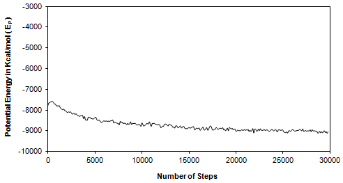
Figure 5: Time Dependence of Potential Energy at Equilibration Stage

STEP V: Production Stage of the System

This stage of MD trajectory is used to sample the structural characteristics and dynamics of the ionic liquids at the desired temperature. The required ensemble i.e NVT, NVE or NPT is chosen to record the system trajectory. Here the initial coordinates are read from final step of equilibration stage. Velocity reassigning or rescaling is now turned off. A new Maxwell distribution of velocities during initialization of production run is created based on the given temperature. The fluctuations in instantaneous temperature and nearly constant total energy (kinetic plus potential energies) are shown in Fig. 6 and 7 respectively. Appendix B,C,D and E provides the input files in NAMD for minimization, heating, equilibration and production step respectively.

Simulation Details
The initial structure of 125 cation and 125 anions was generated through PACKMOL [Martinez and Martinez, 2003] starting with a low density configuration. Then minimization, heating and equilibriation steps were carried out as discussed above. Molecular dynamics simulations in NVT and NPT ensembles were done in NAMD version 2.6. The cell volumes and total energy were monitored until a steady state was reached. The pressure and temperature were controlled using Langevin dynamics along with Nose´-Hoover [Hoover, 1985] barostat with thermostat. The barostat oscillation time and damping time were set to 200 fs and 100 fs respectively. The thermostat damping factor was set at 0.2 ps^-1.All the C-H bonds were held rigid using the SHAKE algorithm [Ryckaert et al., 1977]. The r-RESPA [Tuckerman et al., 1990] multiple time-stepping algorithm was used with a time step of 2 fs for bonded and van der Waals and 4 fs for electrostatic interactions. The dispersion interactions were cut off beyond 20.0 Å. A switching function, initiated at a distance of 18.5 Å, was used to bring the dispersion interactions smoothly to zero at the cutoff distance. Electrostatics were handled by means of a Particle Mesh Ewald (PME) method [Darden et al., 1993] and [Essman et al., 1995] with a grid size of 32.For the cohesive energy density calculations, the ideal gas state was modeled by simulating a single formula unit in an unbounded box in the canonical ensemble. The simulations were conducted at atmospheric pressure (0.98 bar) and at temperatures 298, 323, and 343 K.

Benchmarking System

For ionic liquids all cation intramolecular ( ) and Lennard-Jones parameters ( )are directly taken from the CHARMM 22 force field [Brooks et al.,1983] and used without modification. The simulations are first benchmarked for 1-butyl-3-methylimidaozlium hexafluorophosphate with respect to Morrow and Maginn,2002.
The minimum-energy geometry of the cation and the anion was determined by performing ab initio geometry optimizations on the isolated cation and anion at the HF/6-31G* level of theory using Gaussian 03.The minimization procedure has already been discussed in our earlier module on ab-initio technique so we would not go into the details (Figure 6). The bond lengths as obtained from Quantum Mechanical calculations are compared with those from experimental data and subsequently used in the forcefield calculations [Table 1].