In this section our goal is to derive the response of a LTI system for any arbitrary continuous input x(t). In complete analogy with the discussion on Discrete time analysis we begin by expressing x(t) in terms of impulses. In discrete time we represented a signal in terms of scaled and shifted unit impulses. In continuous time, however the unit impulse function is not an ordinary function (i.e. it is not defined at all points and we prefer to call the unit impulse function a "mathematical object"), it is a generalized function ( it is defined by its effect on other signals) .

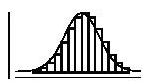
Recall the previous discussion on the development of the unit impulse function. It can be regarded as the idealization of a pulse of width and height 1/.

One can arrive at an expression for an arbitrary input, say x(t) by scaling the height of the rectangular impulse by a factor such that it's value at t coincides with the value of x(t) at the mid-point of the width of the rectangular impulse. The entire function is hence divided into such rectangular impulses which give a close approximation to the actual function depending upon how small the interval is taken to be. For example let x(t) be a signal. It can be approximated as :

The given input x(t) is approximated with such narrow rectangular pulses, each scaled to the appropriate value of x(t) at the corresponding t (which lies at the midpoint of the base of width . This is called the staircase approximation of x(t). In the limit as the pulse-width ( ) approaches zero, the rectangular pulse becomes finer in width and the function x(t) can be represented in terms of impulses by the following expression,

This summation is an approximation. As approaches zero, the approximation increases in accuracy and when delta becomes infinitesimally small, this error becomes zero and the above summation is converted into the following integral expression.

since u(t) = 0 for t < 0 and u(t) = 1 for t > 0. In complete analogy with the development on sampling property of discrete unit impulse we have,

This is known as Sifting Property of the continuous time impulse. Note that the unit impulse puts unit area into zero width.