And finally it takes the following form
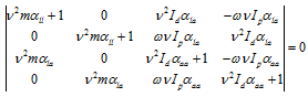
Above determinant will give a polynomial of the eighth degree, however, it can be simplified as
 |
(5.95) |
This gives the same as frequency equation in Section 5.5, which was treated in only one plane. Hence, all the analysis of the quasi-static case will be valid here also.
In matrix form, eigen value problem for the synchronous whirl (the forward and backward whirls) can be obtained as follows. For the forward synchronous whirl, v = ω = ωFcr
(5.96) |
which can be written as
(5.97) |
with
![]()
which is a standard eigen value problem and it will give frequency equation as (on taking determinant of the matrix in equation (5.97))
(5.98) |
From which two critical speeds ωFcr1,2 can be obtained. For the backward synchronous whirl, v = -ω = ωBcr
(5.99) |
where the eigen value problem will be of the same form as equation (5.97). The frequency equation corresponding to this would be
![]()
From which another two critical speeds ωBcr can be obtained. It should be noted from equations (5.97) and (5.99) that the effective mass for the forward whirl is less than the original mass matrix, and for the backward whirl it is more. Hence, the net effect would be to increase in the whirl frequency for the forward whirl and decrease in the whirl frequency for the backward whirl. This particular trend is observed in previous sections also.
5.7 Analysis of Gyroscopic effects with Energy Methods*
Governing differential equations can also be obtained by considering the Hamilton’s principle or Lagrange’s equations (see Chapter 7 for details). The kinetic energy without gyroscopic moment of the disc, as shown in Figure 5.39, is given as
(5.101) |
In Figure 5.39(c) for the y-z plane the gyroscopic moment, ![]() , is in the opposite direction to the angular displacement, φx, in that plane. Hence, it gives rise to the additional kinetic energy, as
, is in the opposite direction to the angular displacement, φx, in that plane. Hence, it gives rise to the additional kinetic energy, as
(5.102) |
Similarly in Figure 5.39(b) for the z-x plane the gyroscopic moment, ![]() , is in the same direction as the angular displacement, φy. Hence, it gives rise to the additional kinetic energy, as
, is in the same direction as the angular displacement, φy. Hence, it gives rise to the additional kinetic energy, as
(5.103) |
Hence, the total kinetic energy of the disc is given as
(5.104) |
Or the gyroscopic term could also be written as (since for conservative system we have ![]() that is
that is ![]() )
)
![]()
The strain energy stored in the shaft is given by
(5.105) |
The Hamilton principle could be used to obtain equations of motion from the kinetic and strain energies, and is expressed as
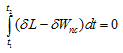 |
(5.106) |
with
| L = T - U | (5.107) |
where L is the Lagrangian function and δWnc is the non-conservative virtual work (for the present case δWnc = 0). On substituting equations (5.104) and (5.105) into equation (5.106), we get
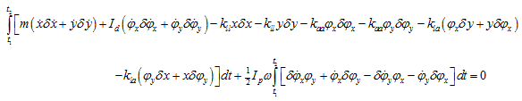 |
(5.108) |
On performing integration by parts with respect to time of the first four and last four terms of equation (5.108), we have
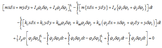 |
(5.109) |
Since the variation is defined with the space, hence all terms, with time dependent limits will vanish. Equation (5.109) can be simplified as
 |
(5.110) |
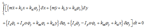
Since δx, δy, δφx and δφy are arbitrary variations, hence we can equate their coefficients in equation (5.110) to be zero
(5.111) |
and
(5.112) |
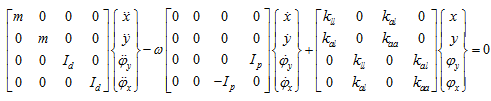
which is same as equation (5.88), obtained by the Newton’s second law. In the matrix form above equations can be written as
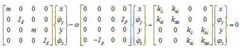
Sometimes the stacking of the vector is different and the for above equation we can have the following form
It would be interesting to obtain the same equations of motion by Lagrange’s equations (refer chapter 7) and it is left to the reader as an exercise.