where ![]() represent vector since displacement has magnitude and phase information. Hence, we can be able to work with complex quantities. Similarly
represent vector since displacement has magnitude and phase information. Hence, we can be able to work with complex quantities. Similarly
|
(13.17) |
We remove the trial mass from plane R and place a trial mass,![]() , in plane L and repeat the test to obtain the measured values
, in plane L and repeat the test to obtain the measured values
|
(13.18) |
and
|
(13.19) |
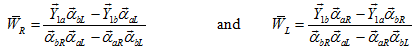
With the help of equations (13.16) to (13.19), we can obtain influence coefficients experimentally. Let the correct balance masses be ![]() in the right and left balancing planes, respectively. Since the original unbalance responses due to residual unbalances are Y1b and Y1a as measured in the right and left planes, we can write
in the right and left balancing planes, respectively. Since the original unbalance responses due to residual unbalances are Y1b and Y1a as measured in the right and left planes, we can write
|
(13.20) |
Correction masses will produce vibration equal and opposite to the vibration due to residual unbalance masses. Hence,

These can be calculated either by a graphical method or analytical method of vectors (complex algebra). We know
which gives
|
(13.20) |
A schematic and a picture of the overall experimental for dynamic balancing of rotor setup are shown in Figs. 13.18 and 13.19, respectively. Fig. 13.20 shows measurement of the phase of the vibration signal, y(t ), with respect to the reference signal, r(t) (or key-phasor). During balancing procedures, the role of reference signal is important since it gives position of a physical mark (i.e., either key-hole or light-reflecting tape) as a spike in the time signal, and other vibration measurements with 1× signal (often narrow-band filters are used to get smooth 1× signal at rotor speed that is the forced response due to residual unbalances) is compared with this reference signal for measurement of the phase (see Fig. 13.20).
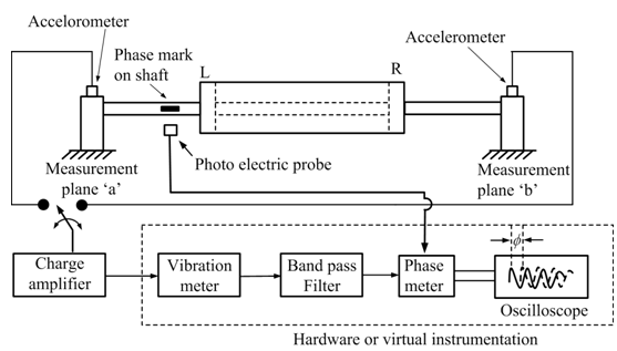
Figure 13.18 A schematic of experimental set-up for the dynamic balancing of a rotor
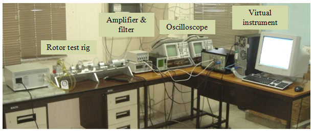
Fig. 13.19 An experimental setup for the dynamic balancing of a rotor test rig