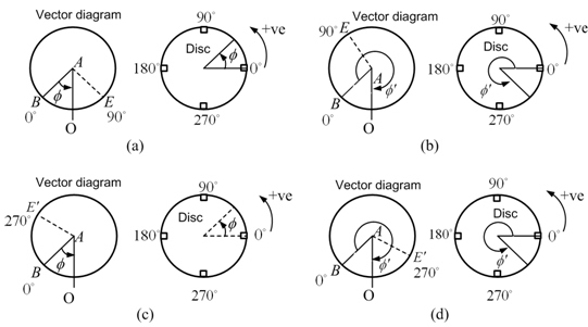
Fig. 13.13 Procedure of obtaining the sense of the angular position of the unbalance mass

In Fig. 13.13(a) the left hand side figure represents the location of the intersection of fourth measurement on the circle (i.e., at E) for trial mass kept at 90⁰ on the disc. This gives the CCW direction as positive for measurement of unbalance angular position, Φ, from 0o location (i.e., AB). The right hand side drawing of Fig. 13.13(a) represents the residual unbalance position, Φ, on the disc location that is CCW direction always (assumed) as positive from 0⁰. In case for the above measurement the intersection of the fourth measurement (i.e., point E) is as shown in Fig. 13.13(b) for the trial mass kept at 90⁰ on the disc then this gives the CW direction as positive for measurement of unbalance angular position, Φ, from 0⁰ location (i.e., AB). The right hand side drawing of Fig. 13.13(b) represents the unbalance position, Φ, on the disc location that is CW direction as positive from 0⁰. Similarly, Figs. 13.13 (c and d) can be interpreted, which are corresponding to measurement taken by placing the trial mass at 270° location on the disc.

The test is repeated by making the cradle pivoted at F₂ and measurements made in plane I. This procedure is also little time consuming and also restricts the mass and size of the rotor. Modern balancing machines use amplitude and phase measurement in two planes for the dynamic balancing of a rigid rotor.

Example 13.3 In the balancing process we make the following observations: (i) a_o= amplitude of vibration of the unbalanced rotor “as is” (ii) a₁ = amplitude with an additional one-unit correction at the location 0 deg and (iii) a₂ = same as a₁ but now at 180 deg.

The ideal rotor, unbalanced only with a unit unbalance (and thus not containing the residual unbalance), will have certain amplitude, which we cannot measure. Call that amplitude x. Let the unknown location of the original unbalance be Φ. Solve x and Φ in terms of   to show that in this answer there is an ambiguity sign and prove that total four runs are necessary to solve the problem completely.

 

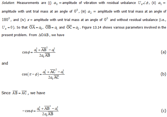
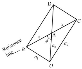
Figure 13.14 Geometrical constructions for determination of residual unbalance