.................................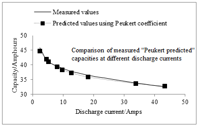
Fig. 2 Showing how closely the Peukert model fits real battery data. In this case the data is from a nominally 42V lead acid Battery
| .........................................................(8) |
Using this, and equation 8 , we can calculate the capacity that the Peukert equation would give us for a range of currents. This has been done with the crosses in Figure 2 . As can be seen, these are quite close to the graph of the measured real values.
The conclusion from equation 4 is that if a current I flows from a battery, then, from the point of view of the battery capacity, the current that appears to flow out of the battery is I k A. Clearly, as long as I and k are greater than 1.0, then I k will be larger than I.
We can use this in a real battery simulation, and we see how the voltage changes as the battery are discharged. This is done by doing a step-by-step simulation, calculating the charge removed at each step. This can be done quite well in EXCEL or MATLAB.
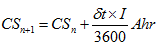
The time step between calculations we will call δt . If the current flowing is I A, then the apparent or effective charge removed from the battery is:
| ...............................................................(9) |
If δt is in seconds, this will be have to be divided by 3600 to bring the units into Amp hours. If CRn is the total charge removed from the battery by the n th step of the simulation, then we can say that:
| ..................................................................(10) |
It is very important to keep in mind that this is the charge removed from the plates of the battery. It is not the total charge actually supplied by the battery to the vehicle’s electrics. This figure, which we could call CS (charge supplied), is given by the formula:
 |
....................................................................(11) |
This formula will normally give a lower figure. As we saw in the earlier sections, this difference is caused by self-discharge reactions taking place within the battery. The depth of discharge of a battery is the ratio of the charge removed to the original capacity. So, at the n th step of a step-by-step simulation we can say that:
 |
.....................................................................(12) |
Where, Cp is the Peukert Capacity, as from equation 11 . This value of depth of discharge can be used to find the open circuit voltage, which can then lead to the actual terminal voltage from the simple equation already given as equation 1 . To simulate the discharge of a battery these equations are ‘run through', with n going from 1, 2, 3, 4, etc., until the battery is discharged. This is reached when the depth of discharge is equal to 1.0, though it is more common to stop just before this, say when DoD is 0.99.
Figure 3 shows the graphs of voltage for three different currents. The voltage is plotted against the actual charge supplied by the battery, as in equation 1 . The power of this type of simulation can be seen by comparing Figure 3 with Fig. 4, which is a copy of the similar data taken from measurements of the real battery.