The Implementation of Flux Weakening
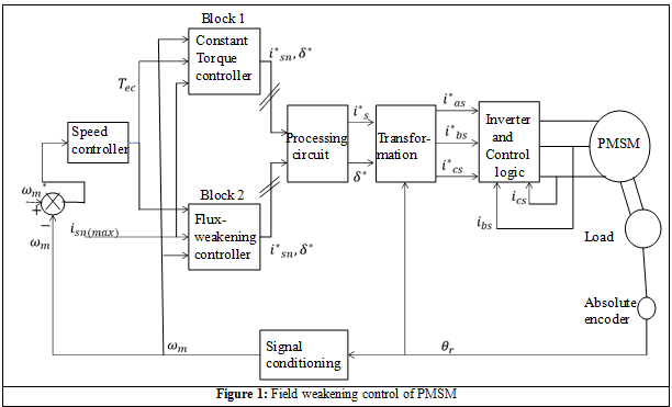
An implementation of the flux weakening control strategy is shown in Figure 1 . From Figure 1 it can be seen that there are two distinct blocks namely:

1. Constant torque mode controller
2. Flux weakening controller

The working of the control strategy is as follows:

1. Based on the error between the reference speed (ω^*_m) and the measured speed (ω_rn), the required torque T_ereq is calculated in the Speed Controller.
2. As long as the measured speed of the motor is less than the base speed (ω_base), the Constant Torque Mode Controller operates. Once the measured speed exceeds the base speed, the Flux Weakening Controller comes into action.
3. The output of the two controllers explained in step ii is the required magnitude of the stator current (I^*_mn) and the load angle (δ^*).
4. Having known the values of I^*_mn and δ^*, the q and d axis currents are calculated using equation 2 in Lecture 25. From the calculated values of  the values of three phase currents are calculated using equation 12 or 13. These thee phase currents are in turn multiplied by base value of the current (I_b) and the required values of the currents are obtained. All these calculations are done in the Transformation Block.
5. The error between and the measured three phase currents is then fed to the DC-AC Controller and the switching logics for the gates are calculated using PWM technique (refer Lecture 16).
6. These switching logic are fed to the DC-AC converter and this produced the required voltage to motor.

The detailed explanation of the Constant Torque Mode Controller and Flux Weakening Controller are given in the subsequent sections.

The Constant Torque Mode Controller
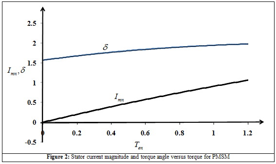
In this block the Optimum torque per ampere control (refer Lecture 25) is implemented. Here, based on T_ereq the values of I^*_mn and δ^* are calculated. This is done by using curve fitting the characteristics for online computation or programming it in the memory of the microcontroller. To understand this consider the PM machine whose parameters are given in Table I. For this machine the Torque (T_e) versus I_mn and δ characteristics are calculated using equation 3a and equation 32 given in Lecture 26 and in Figure 2.The characteristics curves are approximated by third order polynomial and are written as

(17)

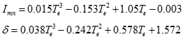
The equations 17and 18 are implemented in form of look-up table in the microcontrollers and their implementation is shown Figure 3.