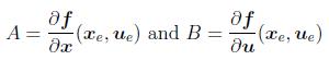
Module 8 : Controllability, Observability and Stability of Discrete Time Systems

Lecture 3 : Revisiting the basics

Note that $ \boldsymbol{f}(\boldsymbol{x}_e, \boldsymbol{u}_e) = 0$. Let

$\displaystyle A = \frac{\partial \boldsymbol{f}}{\partial \boldsymbol{x}} (\boldsymbol{x}_e,\boldsymbol{u}_e)$
(3)


Neglecting higher order terms, we arrive at the linear approximation


$\displaystyle \Delta \boldsymbol{x}(k+1) = A \Delta \boldsymbol{x}(k) + B \Delta \boldsymbol{u}(k)$
(4)

Similarly, if the outputs of the nonlinear system model are of the form


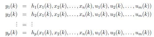
or in vector notation

$\displaystyle \boldsymbol{y}(k) = \boldsymbol{h}(\boldsymbol{x}(k),\boldsymbol{u}(k))$
(5)


then Taylor's series expansion can again be used to yield the linear approximation of the above output equations. Indeed, if we let


$\displaystyle \boldsymbol{y} = \boldsymbol{y}_e + \Delta \boldsymbol{y}$
(6)


then we obtain


$\displaystyle \Delta \boldsymbol{y}(k) = C \Delta \boldsymbol{x}(k) + D \Delta \boldsymbol{u}(k)$

(7)


Example: Consider a nonlinear system
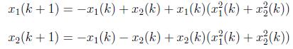
8(a)

8(b)