In this lecture we would discuss Lyapunov stability theorem and derive the Lyapunov Matrix Equation for discrete time systems.

1 Revisiting the basics

Linearization of A Nonlinear System Consider a system

$\displaystyle \boldsymbol{x}(k+1)=\boldsymbol{f}(\boldsymbol{x}(k),\boldsymbol{u}(k))$

where functions are continuously differentiable. The equilibrium point $(\boldsymbol{x}_e,\boldsymbol{u}_e)$ for this system is defined as $\displaystyle \boldsymbol{f}(\boldsymbol{x}_e,\boldsymbol{u}_e)=\boldsymbol{0}$

. What is linearization?
Linearization is the process of replacing the nonlinear system model by its linear counterpart in a small region about its equilibrium point.

. Why do we need it?
We have well stabilised tools to analyze and stabilize linear systems.

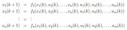
The method: Let us write the general form of nonlinear system $\dot{x}=f(x,u)$ as:

Let $\boldsymbol{u}_e=[u_{1e}\;\;\;u_{2e}\;\;\;\ldots\;\;\;u_{me}]^T$ be a constant input that forces the system to settle into a constant equilibrium state $\boldsymbol{x}_e=[x_{1e}\;\;\;x_{2e}\;\;\;\ldots\;\;\;x_{ne}]^T$ such that $\boldsymbol{f}(\boldsymbol{x}_e,\boldsymbol{u}_e)=\boldsymbol{0}$ holds true.

We now perturb the equilibrium state by allowing: $\boldsymbol{x}=\boldsymbol{x}_e+\Delta \boldsymbol{x}$ and $\boldsymbol{u}=\boldsymbol{u}_e+\Delta \boldsymbol{u}$ . Taylor's expansion yields

$\begin{equation*}\begin{aligned}\Delta \boldsymbol{x}(k+1)=f(\boldsymbol{x}_e+\D... ...{x}_e,\boldsymbol{u}_e) \Delta \boldsymbol{u} + ... \end{aligned}\end{equation*}$

where

$\displaystyle \frac{\partial \boldsymbol{f}}{\partial \boldsymbol{x}} (\boldsym... ...&\cdots&\frac{\partial f_n}{\partial u_m}\end{bmatrix} \right \vert _{x_e, u_e}$

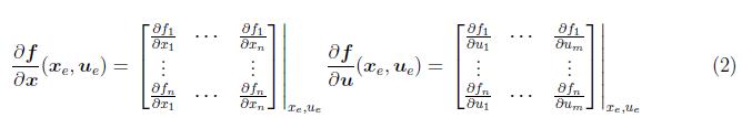are the Jacobian matrices of f with respect to x and u, evaluated at the equilibrium point, $[\boldsymbol{x}_e^T\quad \boldsymbol{u}_e^T]^T$ .