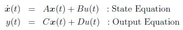
2.1 State Equations of Sampled Data Systems
Let us assume that the following continuous time system is subject to sampling process with an interval of T.
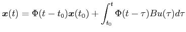
We know that the solution to above state equation is:
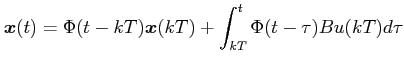
Since the inputs are constants in between two sampling instants, one can write:
which implies that the following expression is valid within the interval
![]() if we consider
if we consider ![]() :
:
Let us denote
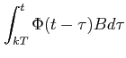 by
by
![]() . Then we can write:
. Then we can write:
If ![]() ,
,
| (4) |