1.1 Correlation between state variable and transfer functions models

The transfer function corresponding to state variable model (1) , when u and y are scalars, is:

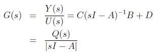(2)

where $\vert sI-A\vert$ is the characteristic polynomial of the system.

1.2 Solution of Continuous Time State Equation

The solution of state equation (1) is given as

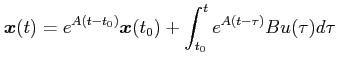
$\displaystyle \boldsymbol{x}(t) = e^{A(t-t_0)}\boldsymbol{x}(t_0)+\int_{t_0}^te^{A(t-\tau)}Bu(\tau)d\tau$

where $e^{At} = \Phi(t)$ is known as the state transition matrix and x(t_o) is the initial state of the system.

2 State Variable Analysis of Digital Control Systems

The discrete time systems, as discussed earlier, can be classified in two types.

1. Systems that result from sampling the continuous time system output at discrete instants only, i.e., sampled data systems.

2. Systems which are inherently discrete where the system states are defined only at discrete time instants and what happens in between is of no concern to us.