Introduction to State Variable Model

In the preceding lectures, we have learned how to design a sampled data control system or a digital system using the transfer function of the system to be controlled. Transfer function approach of system modeling provides final relation between output variable and input variable.

However, a system may have other internal variables of importance. State variable representation takes into account of all such internal variables. Moreover, controller design using classical methods, e.g., root locus or frequency domain method are limited to only LTI systems, particularly SISO (single input single output) systems since for MIMO (multi input multi output) systems controller design using classical approach becomes more complex.

These limitations of classical approach led to the development of state variable approach of system modeling and control which formed a basis of modern control theory.

State variable models are basically time domain models where we are interested in the dynamics of some characterizing variables called state variables which along with the input represent the state of a system at a given time.

State: The state of a dynamic system is the smallest set of variables, xεRⁿ , such that given x(t_o) and u(t), t > t_o, x(t), t > t_o can be uniquely determined.

Usually a system governed by a n^th order differential equation or n^th order transfer function is expressed in terms of n state variables: x₁, x₂,....... x_n.

The generic structure of a state-space model of a n^th order continuous time dynamical system with m input and p output is given by:

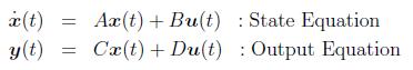(1)

where, x(t) is the n dimensional state vector, u(t) is the m dimensional input vector, y(t) is the p dimensional output vector and AεR^{n x n} , B εR^{n x m,} , CεR^{p x n,}, D εR^{p x m,}