Now,

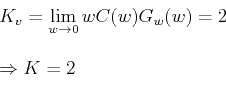
$\begin{displaymath} \begin{array}{l} K_v = \mathop {\lim }\limits_{w \to 0} wC(w)G_w(w) = 2\\ \\ \Rightarrow K = 2 \\ \end{array} \end{displaymath}$

Using MATLAB command ``margin'', phase margin of the system with K = 2 is computed as 31.6° with ω_g = 1.26 rad/sec, as shown in Figure 3.

**Figure 3:** Bode plot of the uncompensated system for Example 2
$\includegraphics[width=4.in]{m5l6fig1a.eps}$

Thus the required phase lead is 50° - 31.6° = 18.4° . After adding a safety margin of 11.6° , $\phi _{\max }$ becomes 30° . Hence

$\displaystyle \alpha = \left( {\frac{{1 - \sin (29^o )}}{{1 + \sin (29^o )}}} \right) = 0.33$

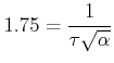
From the frequency response of the system it can be found out that at ω = 1.75 rad/sec, the magnitude of the system is 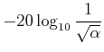$-20 \log_{10} \dfrac{1}{\sqrt \alpha}$ . Thus ω_max = ω_{g_new}= 1.75 rad/sec. This gives

$\displaystyle 1.74 = \frac{1}{{\tau \sqrt \alpha }}$
Or, $\displaystyle \tau = \frac{1}{{1.74\sqrt{0.33}}} = 1$

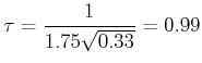
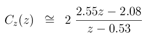
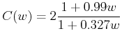
Thus the controller in w-plane is

$\displaystyle C(w) = 2 \frac{1+w}{1+0.33 w}$

The Bode plot of the compensated system is shown in Figure 4.

**Figure 4:** Bode plot of the compensated system for Example 2
$\includegraphics[width=4.2in]{m5l6fig1b.eps}$

Re-transforming the above controller into z -plane using the relation 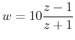$w=10\dfrac{z-1}{z+1}$ , we get the controller in z -plane, as