Critical value of K can be found out from the magnitude criterion.

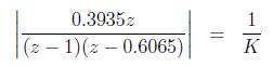
Critical gain corresponds to point . Thus

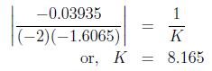
Figure 2 shows the root locus of the system for K = 0 to K =10. Two root locus branches start from two open loop poles at K = 0. If we further increase K one branch will go towards the zero and the other one will tend to infinity. The blue circle represents the unit circle. Thus the stable range of K is 0 < K < 8.165.

$\includegraphics[width=12cm, height=8cm]{rl1_mt.eps}$

Figure 2: Root Locus when T=0.5 sec

If T = 1 sec,

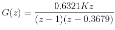$\displaystyle G(z)=\frac{0.6321 Kz}{(z-1)(z-0.3679)}$

Break away/ break in points:
$z^{2}=0.3679 \Rightarrow z_{1}=0.6065$ and $z_{2}=-0.6065$ Critical gain $(K_{c})=4.328$ Figure 3 shows the root locus for K = 0 to K = 10. It can be seen from the figure that the3 radius of the inside circle reduces and the maximum value of stable K also decreases to K = 4.328 .

$\includegraphics[width=12cm, height=8cm]{rl2_mt.eps}$

Figure 3: Root Locus when T=1 sec

Similarly if T = 2 sec,

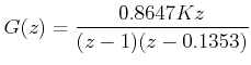$\displaystyle G(z)=\frac{0.8647 Kz}{(z-1)(z-0.1353)}$

One can find that the critical gain in this case further reduces to 2.626.