So far we have discussed about the modelling of a discrete time system by pulse transfer function, various stability tests and time domain performance criteria. The main objective of a control system is to design a controller either in forward or in feedback path so that the closed loop system is stable with some desired performance. Two most popular design techniques for continuous time LTI systems are using root locus and frequency domain methods.
1 Design based on root locus method
- • The effect of system gain and/or sampling period on the absolute and relative stability of the closed loop system should be investigated in addition to the transient response characteristics. Root locus method is very useful in this regard.
• The root locus method for continuous time systems can be extended to discrete time systems without much modifications since the characteristic equation of a discrete control system is of the same form as that of a continuous time control system.
In many LTI discrete time control systems, the characteristics equation may have either of the following two forms.
| 0 | |||
| 0 |
To combine both, let us define the characteristics equation as:
| (1) |
where, ![]() or
or ![]() .
. ![]() is popularly known as the loop pulse transfer function. From equation (1), we can write
is popularly known as the loop pulse transfer function. From equation (1), we can write
![]()
Since ![]() is a complex quantity it can be split into two equations by equating angles and magnitudes of two sides. This gives us the angle and magnitude criteria as
is a complex quantity it can be split into two equations by equating angles and magnitudes of two sides. This gives us the angle and magnitude criteria as
Angle Criterion: ![]()
Magnitude Criterion: ![]()
The values of z that satisfy both criteria are the roots of the characteristics equation or close loop poles. Before constructing the root locus, the characteristics equation ![]() should be rearranged in the following form
should be rearranged in the following form
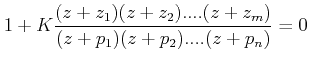 |
where ![]() 's and
's and ![]() 's are zeros and poles of open loop transfer function, m is the number of zeros n is the number of poles.
's are zeros and poles of open loop transfer function, m is the number of zeros n is the number of poles.