Solution:

$\displaystyle \frac{C(z)}{R(z)}$

$\displaystyle =$

$\displaystyle \frac{G(z)}{1+GH(z)}$

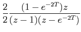
Since the feedback transfer function is 1,

$\displaystyle G(z)=GH(z)$	$\displaystyle =$	$\displaystyle z \left[\frac{2}{s(s+2)}\right]$
	$\displaystyle =$	$\displaystyle \frac {2}{2} \frac{(1-e^{-2T})z}{(z-1)(z-e^{-2T})}$
	$\displaystyle =$	$\displaystyle \frac {2}{2} \frac{(1-e^{-2T})z}{(z-1)(z-e^{-2T})}$
$\displaystyle \Rightarrow \frac {C(z)}{R(z)}$	$\displaystyle =$	$\displaystyle \frac {0.18z}{z^{2}-1.64z+0.82}$

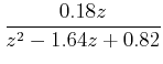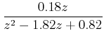
So, the characteristics equation of the system is $z^{2}-1.64z+0.82=0$ .

1.2 Causality and Physical Realizability

In a causal system, the output does not precede the input. In other words, in a causal system, the output depends only on the past and presents inputs, not on the future ones.

The transfer function of a causal system is physically realizable, i.e., the system can be realized by using physical elements.

For a causal discrete data system, the power series expansion of its transfer function must not contain any positive power in z Positive power in z indicates prediction. Therefore, in the transfer function (6), n must be greater than or equal to m.

: m = n $\Rightarrow$ proper transfer function
m < n $\Rightarrow$ strictly proper Transfer function