1. Pluse Transfer Function of Closed Loop Systems

We know that various advantages of feedback make most of the control systems closed loop in nature. A simple single loop system with a sampler in the forward path is shown in Figure 1.

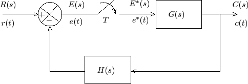
$\begin{figure}\centering\vspace{0.5cm} \input{m2l4f1.pstex_t}\end{figure}$
Figure 1: Block diagram of a closed loop system with a sampler in the forward path

The objective is to establish the input-output relationship. For the above system, the output of the sampler is regarded as an input to the system. The input to the sampler is regarded as another output. Thus the input-output relations can be formulated as

$\displaystyle E(s)$	$\displaystyle =$	$\displaystyle R(s)-G(s)H(s)E^{*}(s)$	(1)
$\displaystyle C(s)$	$\displaystyle =$	$\displaystyle G(s)E^{*}(s)$	(2)

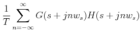
Taking pulse transform on both sides of (1),

$\displaystyle E^{*}(s)=R^{*}(s)-GH^{*}(s)E^{*}(s)$

(3)

where

$\displaystyle GH^{*}(s)$	$\displaystyle =$	$\displaystyle [G(s)H(s)]^{*}$
	$\displaystyle =$	$\displaystyle \frac{1}{T}\sum_{n=-\infty}^{\infty}G(s+jnw_{s})+(s+jnw_{s})$