Module 2 : Modeling Discrete Time Systems by Pulse Transfer Function

Lecture 4 : Pulse Transfer Functions of Closed Loop Systems

We can write from equation (3),

$\displaystyle E^{*}(s)$
$\displaystyle =$ $\displaystyle \frac {R^{*}(s)}{1+GH^{*}(s)}$  
$\displaystyle \Rightarrow C(s)$
$\displaystyle =$ $\displaystyle G(s)E^{*}(s)$  
  $\displaystyle =$ $\displaystyle \frac {G(s)R^{*}(s)}{GH^{*}(s)}$  

Taking pulse transformation on both sides of (2)

$\displaystyle C^{*}(s)$
$\displaystyle =$ $\displaystyle [G(s)E^{*}(s)]^{*}$  
  $\displaystyle =$ $\displaystyle G^{*}(s)E^{*}(s)$  
  $\displaystyle =$ $\displaystyle \frac {G^{*}(s)R^{*}(s)}{1+GH^{*}(s)}$  


% latex2html id marker 463
$\displaystyle \therefore \; \frac {C^{*}(s)}{R^{*}(s)}$
$\displaystyle =$$\displaystyle \frac{G^{*}(s)}{1+GH^{*}(s)}$    
$\displaystyle \Rightarrow \frac {C(z)}{R(z)}$
$\displaystyle =$$\displaystyle \frac{G(z)}{1+GH(z)}$    

where $ GH(z)=Z[G(s)H(s)]$.

$ $
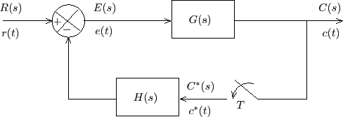
Now, if we place the sampler in the feedback path, the block diagram will look like the Figure 2.

Figure 2: Block diagram of a closed loop system with a sampler in the feedback path
\begin{figure}\centering\vspace{0.5cm}
\input{m2l4f2.pstex_t}\end{figure}