Module 2 : Modeling Discrete Time Systems by Pulse Transfer Function

Lecture 4 : Pulse Transfer Functions of Closed Loop Systems

The corresponding input output relations can be written as:

$\displaystyle E(s)$
$\displaystyle =$ $\displaystyle R(s)- H(S)C^{*}(s)$ (4)

$\displaystyle C(s)$
$\displaystyle =$ $\displaystyle =G(s)R(s)-G(s)H(s)C^{*}(s)$ (5)

$ $
Taking pulse transformation of equations (4) and (5)

$\displaystyle E^{*}(s)$
$\displaystyle =$ $\displaystyle R^{*}(s)-H^{*}(s)C^{*}(s)$  
$\displaystyle C^{*}(s)$
$\displaystyle =$ $\displaystyle GR^{*}(s)-GH^{*}(s)C^{*}(s)$  
where,$\displaystyle \;\;
GR^{*}(s)$
$\displaystyle =$ $\displaystyle [G(s)R(s)]^{*}$  
$\displaystyle GH^{*}(s)$
$\displaystyle =$ $\displaystyle [G(s)H(s)]^{*}$  

can be written as

$\displaystyle C^{*}(s)$
$\displaystyle =$ $\displaystyle \frac {GR^*(s)}{1+GH^{*}(s)}$  
$\displaystyle \Rightarrow C(z)$
$\displaystyle =$ $\displaystyle \frac {GR(z)}{1+GH(z)}$  


We can no longer define the input output transfer function of this system by either $ \dfrac {C^{*}(s)}{R^{*}(s)}$ or $ \dfrac{C(z)}{R(z)}$. Since the input $ r(t)$ is not sampled, the sampled signal $ r^*(t)$ 
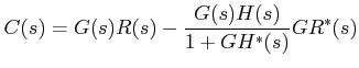
does not exist. The continuous-data output $ C(s)$ can be expressed in terms of input as.

$\displaystyle C(s)=G(s)R(s)-\frac{G(s)H(s)}{1+GH^{*}(s)}GR^{*}(s)$