It may be noted that along with 0 and 1, three more notations namely, D, and X are used. D is used to represent 1/0—i.e., under normal condition the net has value 1 and 0 under presence of a fault. Similarly, represents 0/1. X is used to represent the case when the signal value of a net is unknown. The use of more notations allows determination of signal values for both normal and faulty circuits in one pass. Since a test pattern requires that a difference be maintained between the two circuits, it is computationally fastest to represent both circuits in the algebra, rather than one of them at a time. Figure 2 illustrates two input AND gates where the input/outputs are marked using notations from Roth’s 5-valued algebra.

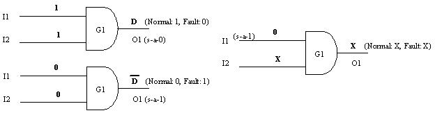
Figure 2. Example to illustrate Roth’s five value algebra
Logical operations using Roth’s 5-valued algebra is very similar to Boolean algebra, only we need two Boolean operations when D or is one of the inputs. Some examples are as follows

............• 1 AND D = D; 1 AND 1/0 involves two computations—(i) 1 AND 1=1, (ii) 1 AND 0=0.

............• 0 OR = ; 0 OR 0/1 involves two computations—(i) 0 OR 0=0, (ii) 0 OR 1=1.

............• NOT() =D; NOT(0/1) involves two computations—(i) NOT(0)=1, (ii) NOT(1)=0.

When one input is X in logical operation then output is also X, if others inputs are non controlling; else output is determined by the controlling input. Some examples are given below

X AND 1 =X; 1 is non controlling in AND logic
X AND 0 =0; 0 is controlling in AND logic

4.Types of ATPG algorithms

4.1 Exhaustive

Testing by “exhaustive” technique implies applying all input combinations and checking for “functional” correctness. As already discussed in last module, for an n-input circuit, an exhaustive test technique would require 2ⁿ input combinations. Considering the time required for exhaustive testing, it is infeasible for circuits with more than about 15 inputs. So exhaustive testing techniques are not used in ATPG.

4.2 Random

As elaborated in the last module, random ATPG basically involves three steps:

Generate a random pattern
Determine how many faults are detected by the random pattern (fault simulation)
Continue the above two steps till no (or few) new faults are detected by the random pattern.

Random patterns can detect “easy to test faults” and the algorithm being fast, it is applied at initial phases of ATPG. Also discussed before, heart of ATPG by random patterns are fault simulation algorithms. We saw four major fault simulations algorithms in the last module namely, sequential, parallel, concurrent and deductive. However, for the faults which cannot be detected by random patterns, we need deterministic ARPG techniques. Now we will see two such types of algorithms (i) symbolic difference and (ii) path sensitization.

4.3 Symbolic Difference

ATPG by symbolic difference is basically based on well-known Shannon’s expansion theorem. Let us explain this by an example. Consider an arbitrary Boolean function as.By Shannon’s expansion rule, the function can be expanded about any variable x₁ say, as = .