Information about these (remaining) gates are retained from the << input I1=1,I2=1; retaining this information over change in input patters is the main advantage of concurrent fault simulation .

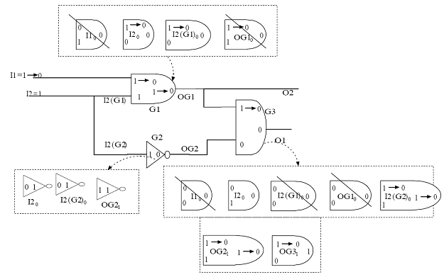
Figure 18. Gates deleted if input changes from I1=1, I2=1 to I1=0, I2=1 (example of the circuit in Figure 17)

The story is not yet over. As some gates get eliminated from the affective list when input pattern changes, also some new gates get added to the list. Figure 19 shows the remaining affected gates and the ones added after change in input. For example, for s-a-1 fault at I1, the gate I1₁ gets added to the list of G1, because first input and output of I1₁ is different compared to G1. Similarly, another gate for s-a-1 fault at OG1 gets added to the list of G1. So affected gate list of G1 has four gates. G1 drives primary output OG1 and outputs of the affected gates I1₁ and OG1₁ are different compared to G1. So s-a-1 in I1 and s-a-1 at OG1 are detected by input 11=0,I2=1. Similarly, in case of primary output O1, s-a-1 fault in OG3 is detected by 11=0,I2=1.

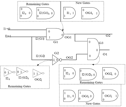
Figure 19. Remaining affected gates and the ones added after change in input.

To conclude, fault simulation algorithms help to determine patters that can test a subset of faults in a circuit. Broadly speaking, after about 90% of faults being detected by random patters and fault simulation, we need to go for ATPG by sensitization–propagation -justification approach. Now, if there was a scheme that could tell which 90% of faults are easy to test (by random patterns) and which are difficult to test, then fault simulation algorithms could be more focused. In other words, fault simulation algorithms would stop when most of the easy faults were covered. In the >> lecture we would see an approximate and fast algorithm, which predicts which faults are easy to test and which are difficult.