3. Binary Decision Diagrams

From the example illustrated in the last section, it may be noted that BDT cannot be generated within practical time lines for a reasonably complex circuit. The main reason is the exponential number of nodes in a BDT with respect to number of inputs. However, it may be noted that there are many redundant nodes in the BDT; simply, in the leaf level we can have one node with “0” and the other with “1” and redirect paths from the nodes of leaf level -1 accordingly. Similarly, this reduction is carried out at all layers till the root.

Broadly speaking, a Binary Decision Diagram (BDD) is a directed acyclic graph representation of the Boolean expression which cannot further be reduced my eliminating redundant nodes. In other words, just like BDT, BDD is an acyclic graph representation of a Boolean expression but unlike BDT, it does not comprise any redundant node either in the leaf or the non-leaf level. So BDD is called Reduced BDD (RBDD).

The reduction from BDT to RBDD is done using three rules.

R1: Removing of duplicate terminals (leaf nodes): If a BDD contains more than one terminal 0-node, then we redirect all edges which point to such 0-node to just one of them and other 0-node can be removed. Similarly we do with 1-node also.
R2: Removal of duplicate non terminals (internal nodes): If two distinct nodes n and m in the RBDD are the roots of structurally identical sub-BDDs, then we eliminate one of them, say m , and redirect all its incoming edges to the other one (node n )
R3: Removal of Redundant test: If both outgoing edges of a node n point to the same node m , then we eliminate the node n , and point all its incoming edges to m .

After application of Rule R1, Rule R2 and Rule R3 repeatedly we get the reduced BDD (from BDT). A BDD is said to be reduced if none of the above rules can be applied further. (i.e., no more reduction is possible).

Now we illustrate application of the above three rules for the BDT of Figure 2.

Figure 3 illustrates the intermediate BDD when R1 is applied to the BDT of Figure 2. It may be noted that there is only one leaf node with “0” and another one with “1”. From Figure 2 it may be observed that the path from root to leaf node corresponding a=b=c=d=0 reaches a leaf node with “0”. Also the path from corresponding to a=b=c=0; d=1reaches a leaf node with “0”. Now as there is a single node at leaf level with “0” in the RBDD (Figure 3) both the paths corresponding toa=b=c=d=0 anda=b=c=0; d=1 has been redirected the single “0” leaf node. Similarly, redirection of all paths in Figure 3 can be explained.

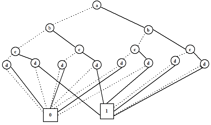
Figure 3. Removal of Duplicate Terminals (Leaf Nodes)

Figure 4 illustrates the intermediate BDD when R2 is applied to the (intermediate) BDD of Figure 3. From Figure 5 it may be noted that the sub-BDDs enclosed by polygons are structurally identical. So we retain only one of them and redirect edges incoming to the eliminated sub-BDD to the one being retained; resulting intermediate BDD is shown in Figure 6. When R2 is applied to all structurally identical sub-BDDs of Figure 3 we obtain the BDD of Figure 4.