![1- t
ϵ = 2 [h + h ],](main835x.png)
In the previous chapters, we mastered the basic concepts of strain and stress along with the four basic equations, namely, the strain-displacement relation, compatibility condition, constitutive relation and the equilibrium equations. We are now in a position to find the stresses and displacement throughout the body - in the interior as well as in its boundary - given the displacement over some part of the boundary of the body and the traction on some other part of the boundary. Usually the part of the boundary where traction is specified, displacement would not be given and vice versa. In this course we shall formulate the boundary value problem for a body made up of isotropic material obeying Hooke’s law and deforming in such a manner that the relative displacement between its particles is small1 . Then, we discuss three strategies to solve this boundary value problem.
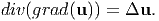
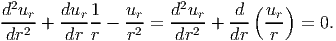
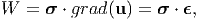
Before we endeavor on the formulation of the boundary value problem and discuss strategies to solve it, we recollect and record the basic equations. If u represents the displacement that the particles undergo from a stress free reference configuration to the deformed current configuration with the deformation taking place due to application of the traction on the boundary, then we define the linearized strain as,
|
| (7.1) |
where, h = grad(u). The equation (7.1) is called as the strain displacement relation. The constitutive relation that relates the stress to the strain that is to be used in this course is the Hooke’s law. The various forms of the same Hooke’s law that would be used is recorded:
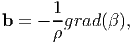
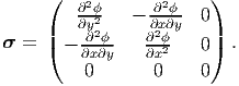
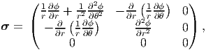
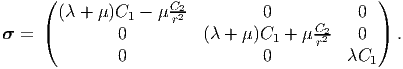
where σ is the Cauchy stress, λ and μ are Lamè constants and E is the Young’s modulus and ν is the Poisson’s ratio. The conservation of linear momentum equation,
 | (7.5) |
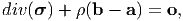
where ρ is the density, b is the body force per unit mass and a is the acceleration, for our purposes here reduces to:
 | (7.6) |
since we have ignored the body forces and look at configurations that are in static equilibrium under the action of the applied static traction. That is the displacement is assumed not to depend on time. It is appropriate that we discuss these assumptions in some detail. By ignoring the body forces we are ignoring the stresses that arise in the body due to its own mass. Since, these stresses are expected to be much small in comparison to the stresses induced in the body due to traction acting on its boundary and these stresses practically do not vary over the surface of the earth, ignoring the body forces is justifiable. In the same spirit, all that we require is that the magnitude of acceleration be small, if not zero.
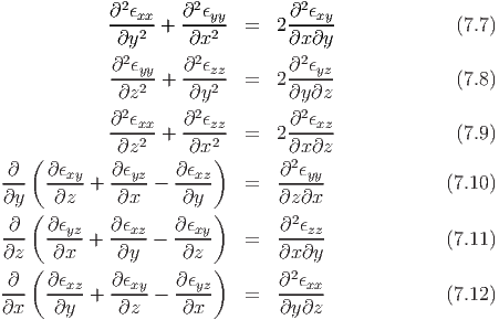
Finally, we document the compatibility conditions; the conditions that ensures the existence of a smooth displacement field given a strain field:
Formulation of the boundary value problem involves specification of the geometry
of the body, the constitutive relation and the boundary conditions. To elaborate,
we have to define the region of the Euclidean point space the body occupies in the
reference configuration, which is denoted by  . For example, the body might
occupy a region that is a unit cube, then using Cartesian coordinates the body is
defined as = {(X,Y,Z)|0 ≤ X ≤ 1, 0 ≤ Y ≤ 1, 0 ≤ Z ≤ 1}. Alternatively, the
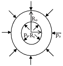
body might be the annular region between two annular cylinders of radius Ro and
Ri and height H, then using cylindrical polar coordinates the body may
be defined as = {(R, Θ,Z)|Ri ≤ R ≤ Ro, 0 ≤ Θ ≤ 2π, 0 ≤ Z ≤ H}.
The boundary of the body, denoted as ∂ is a surface that encloses the
body. For illustration, in the cube example, the surface is composite of 6
different planes, defined by X = 0, X = 1, Y = 0, Y = 1, Z = 0 and
Z = 1 respectively and in the annular cylinder example the surface is
composed of 4 different planes, defined by R = Ri, R = Ro, Z = 0, Z =
H.
. For example, the body might
occupy a region that is a unit cube, then using Cartesian coordinates the body is
defined as = {(X,Y,Z)|0 ≤ X ≤ 1, 0 ≤ Y ≤ 1, 0 ≤ Z ≤ 1}. Alternatively, the
body might be the annular region between two annular cylinders of radius Ro and
Ri and height H, then using cylindrical polar coordinates the body may
be defined as = {(R, Θ,Z)|Ri ≤ R ≤ Ro, 0 ≤ Θ ≤ 2π, 0 ≤ Z ≤ H}.
The boundary of the body, denoted as ∂ is a surface that encloses the
body. For illustration, in the cube example, the surface is composite of 6
different planes, defined by X = 0, X = 1, Y = 0, Y = 1, Z = 0 and
Z = 1 respectively and in the annular cylinder example the surface is
composed of 4 different planes, defined by R = Ri, R = Ro, Z = 0, Z =
H.
In this course, at least, the constitutive relation is known; it is Hooke’s law for isotropic materials. In real life problem, the weakest link in the formulation of the boundary value problem is the constitutive relation.
Then finally one needs to prescribe boundary conditions. These are specifications of the displacement or traction on the surface of the body. Depending on what is prescribed on the surface, there are four type of boundary conditions. They are
Once, the geometry of the body, constitutive relations and boundary conditions are prescribed then finding the Cauchy stress and displacement over the entire region of the body such that the displacement is continuous and differentiable over the entire region occupied by the body and the stress computed using this displacement field from the constitutive relation satisfies the equilibrium equations is called as solving the boundary value problem. If for a given geometry of the body, constitutive relations and boundary conditions, there exists only one displacement and stress field as a solution to the boundary value problem then the solution to the boundary value problem is said to be unique.
Now it is appropriate to make a few comments regarding the choice of the independent variable for the boundary value problem. That is, when we say the region occupied by the body, we should have been more specific and said whether this is the region occupied by the body in the reference or current configuration. As described in section 3.4 of chapter 3, the displacement and the stresses can be given an Eulerian or Lagrangian description, i.e.,
 | (7.13) |
In this course, to be specific, we follow the Eulerian description of these fields. That is we use the region occupied by the body in the current configuration as the spatial domain of the boundary value problem. However, this domain is not known a priori. Therefore, we approximate the region occupied by the body in the current configuration with the region occupied by the body in the reference configuration. This approximation is justified, since we are interested only in problems where the components of the gradient of the displacement field are small and the magnitude of the displacement is also small. Then, one might ponder as to why we cannot say we are following the Lagrangian description of these fields. In chapter 5 section 5.4.1, we showed that the conservation of linear momentum takes different forms depending on the description of the stress field. The equation used here (7.5) is derived assuming Eulerian or spatial description of the stress field. If we use (5.46) instead of (7.5) then we would have said we are following Lagrangian description of these fields. Following Lagrangian description also, we would obtain the same governing equations if we assume that the components of the gradient of the deformation field are small and the magnitude of the displacement is small; but we have to do a little more algebra than saying upfront that we are following an Eulerian or spatial description.
Depending on the boundary condition specified the solution can be found using one of the following two techniques. Outline of these methods is presented next.
Here we take the displacement field as the basic unknown that need to be determined. Then using this displacement field we find the strain using the strain displacement relation (7.1). The so computed strain is substituted in the constitutive relation written using Lamè constants (7.2) to obtain
![[ ]
σ = λdiv(u)1 + μ grad(u ) + grad (u)t ,](main841x.png) | (7.14) |
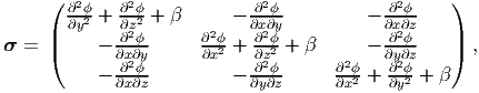
where we have used the definition of divergence operator, (2.208) and the property of the trace operator (2.67). Substituting (7.14) in the reduced equilibrium equations, under the assumption that body forces can be ignored and the body is in static equilibrium, (7.5) we obtain
 | (7.15) |
where we have used equation (3.31) to write the acceleration in terms of the
displacement and  E denotes the total time derivative. In addition, to obtain
the equation (7.15), we have used the following identities:
E denotes the total time derivative. In addition, to obtain
the equation (7.15), we have used the following identities:
 | (7.16) |
 | (7.19) |
 | (7.20) |
 | (7.21) |
Thus, we obtain (7.15) by substituting successive substitution of equations (7.17) through (7.21) in (7.16).
In order to simplify equation (7.15), we make the following assumptions:
In lieu of these assumptions, equation (7.15) reduces to
 | (7.22) |
If body forces cannot be ignored but the other two assumptions hold, then (7.15) reduces to
 | (7.23) |
In this course, we attempt to find the displacement field that satisfies (7.22) along with the prescribed boundary conditions. We compute the stress field corresponding to the determined displacement field, using equation (7.2) where the strain is related to the displacement field through equation (7.1). We illustrate this method in section 7.4.1.
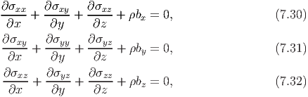
Here we use stress as the basic unknown that needs to be determined. This method is applicable only for cases when the inertial forces (ρa) can be neglected. Since, we have assumed stress as the basic unknown, we want to express the compatibility conditions (7.7) through (7.12) in terms of the stresses. For this we compute the strains in terms of the stresses using the constitutive relation (7.4) and substitute in the compatibility conditions to obtain the following 6 equations:
where we have assumed that the body is homogeneous and hence Young’s modulus, E and Poisson’s ratio, ν do not vary spatially. Now, we have to find the 6 components of the stress such that the 6 equations (7.24) through (7.29) holds along with the three equilibrium equations where bi’s are the Cartesian components of the body forces. The above equilibrium equations (7.30) through (7.32) are obtained from (7.5) by setting a = o. If the body forces could be obtained from a potential, β =  (x,y,z) called as
the load potential, as
(x,y,z) called as
the load potential, as
 | (7.33) |
then the Cartesian components of the Cauchy stress could be obtained from a
potential, ϕ =  (x,y,z) called as the Airy’s stress potential and the load
potential, β as,
(x,y,z) called as the Airy’s stress potential and the load
potential, β as,
 | (7.34) |
so that the equilibrium equations (7.30) through (7.32) is satisfied for any choice of ϕ. Substituting for the Cartesian components of the stress from equation (7.34) in the compatibility equations (7.24) through (7.29) and simplifying we obtain:
Thus, a potential that satisfies equations (7.35) through (7.40) and the prescribed boundary conditions is said to be the solution to the given boundary value problem. Once the Airy’s stress potential is obtained, the stress field could be computed using (7.34). Using this stress field the strain field is computed using the constitutive relation (7.4). From this strain field, the smooth displacement field is obtained by integrating the strain displacement relation (7.1).
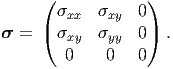
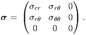
Next, we specialize the above stress formulation for the plane stress case. Without loss of generality, let us assume that the Cartesian components of this plane stress state is
 | (7.41) |
Further, let us assume that body forces are absent and that the Airy’s stress
function depends on only x and y. Thus, β = 0 and ϕ = (x,y). Note that this
assumption for the Airy’s stress function does not ensure σzz = 0, whenever
 +
+  ≠ 0. Hence, plane stress formulation is not a specialization of the general
3D problem. Therefore, we have to derive the governing equations again following
the same procedure.
≠ 0. Hence, plane stress formulation is not a specialization of the general
3D problem. Therefore, we have to derive the governing equations again following
the same procedure.
Since, we assume that there are no body forces and the Airy’s stress function depends only on x and y, the Cartesian components of the stress are related to the Airy’s stress function as,
 | (7.42) |
Substituting for stress from equation (7.42) in the constitutive relation (7.4) we obtain,
![( ∂2ϕ ∂2ϕ ∂2ϕ )
∂y2 - ν∂x2 - (1 + ν)∂x∂y 0
ϵ = -1 || - (1 + ν) ∂2ϕ ∂2ϕ2 - ν∂2ϕ2 0 || .
E ( ∂x∂y ∂x ∂y [ 2 2 ])
0 0 - ν ∂∂ϕx2 + ∂∂ϕy2](main863x.png) | (7.43) |
Substituting for strain from equation (7.43) in the compatibility condition (7.7) through (7.12), the non-trivial equations are
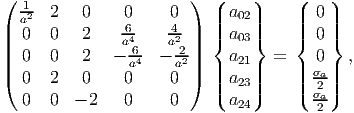
Now, for equations (7.45) through (7.47) to hold,
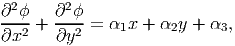 | (7.48) |
where αi’s are constants. Differentiating equation (7.48) with respect to x twice and adding to this the result of differentiation of equation (7.48) with respect to y twice, we obtain equation (7.44). Thus, for equations (7.44) through (7.47) to hold it suffices that ϕ satisfy equation (7.48) along with the prescribed boundary conditions. Comparing the expression for ϵzz in equation (7.43) and the requirement (7.48) arising from compatibility equations (7.8), (7.9) and (7.11) is a restriction on how the out of plane normal strain can vary, i.e., ϵzz = 1x + 2y + 3, where i’s are some constants. Hence, this requirement that ϕ satisfy equation (7.48) does not lead to solution of a variety of boundary value problems. Due to Poisson’s effect plane stress does not lead to plane strain and vice versa, resulting in the present difficulty. To overcome this difficulty, it has been suggested that for plane problems one should use the 2 dimensional constitutive relations, instead of 3 dimensional constitutive relations that we have been using till now.
Since, the constitutive relation is 2 dimensional, plane stress implies plane strain and the three independent Cartesian components of the plane stress and strain are related as,
![1 1 (1 + ν)
ϵxx = --[σxx - νσyy], ϵyy = --[σyy - ν σxx], ϵxy = -------σxy.
E E E](main866x.png) | (7.49) |
Inverting the above equations we obtain
![E E E
σxx = -----2 [ϵxx + ν ϵyy], σyy = -----2-[ϵyy + νϵxx], σxy = ------- ϵxy.
1 - ν 1 - ν (1 + ν)](main867x.png) | (7.50) |
By virtue of using (7.49) to compute the strain for the plane state of stress given in equation (7.42), the only non-trivial restriction from compatibility condition is (7.7) which requires that
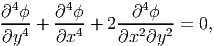 | (7.51) |
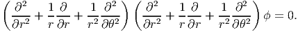
Equation (7.51) is called as the bi-harmonic equation. Thus, for two dimensional problems formulated using stress, one has to find the Airy’s stress potential that satisfies the boundary conditions and the bi-harmonic equation (7.51). Then using this stress potential, the stresses are computed using (7.42). Having estimated the stress, the strain are found from the two dimensional constitutive relation (7.49). Finally, using this estimated strain, the strain displacement relation (7.1) is integrated to obtain the smooth displacement field. We study bending problems in chapter 8 using this approach.
Recognize that equation (7.51) is nothing but Δ(Δ(ϕ)) = 0, where Δ(⋅) is the Laplacian operator.
Next, we would like to formulate the plane stress problem in cylindrical polar coordinates. Let us assume that the cylindrical polar components of this plane stress state is
 | (7.52) |
Further, let us assume that body forces are absent and that the Airy’s stress
function depends on only r and θ, i.e. ϕ =  (r,θ). For this case, the Cauchy stress
cylindrical polar components are assumed to be
(r,θ). For this case, the Cauchy stress
cylindrical polar components are assumed to be
 | (7.53) |
so that it satisfies the static equilibrium equations in the absence of body forces, equation (7.6). Then, using a 2 dimensional constitutive relation, the cylindrical polar components of the strain are related to the cylindrical polar components of the stress through,
![ϵrr = 1-[σrr - ν σθθ], ϵθθ = 1-[σθθ - ν σrr], ϵrθ = (1-+-ν-)σrθ.
E E E](main872x.png) | (7.54) |
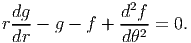
As shown before, the only non-trivial restriction from compatibility condition in 2 dimensions is (7.7) and this in cylindrical polar coordinates takes the form,
![2 2 2
∂-ϵθθ + 1-∂--ϵrr + -2 [ϵrr - ϵθθ] = 2-∂-ϵrθ.
∂r2 r2 ∂θ2 r2 r ∂r∂θ](main873x.png) | (7.55) |
Substituting equation (7.54) and (7.53) in (7.55) and simplifying we obtain,
 | (7.56) |
A general periodic solution to the bi-harmonic equation in cylindrical polar coordinates, (7.56) is
![2 2 [ 2 2 ]
ϕ = a01+a02 ln(r)+a03r +a04r ln(r)+ b01 + b02ln(r) + b03r + b04r ln(r) θ
[ a13 3 ]
+ a11r + a12rln(r) + r + a14r + a15rθ + a16rθ ln (r) cos(θ)
[ ]
+ b11r + b12r ln(r) + b13 + b14r3 + b15rθ + b16rθln(r) sin(θ)
r
∞∑ [ ]
+ an1rn + an2r2+n + an3r- n + an4r2- n cos(nθ)
n=2
∑∞
+ [b rn + b r2+n + b r-n + b r2-n]sin(nθ),
n1 n2 n3 n4
n=2](main875x.png) | (7.57) |
Having formulated the boundary value problem and seen at techniques to solve it, in this section we illustrate the same by solving some standard boundary value problems.
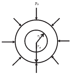
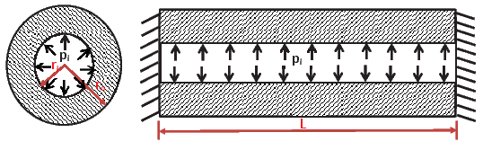
In the first boundary value problem that is of interest, the body is in the form
of an annular cylinder as shown in the figure 7.1. We use cylindrical polar
coordinates to study this problem. Consequently, the body in the reference
configuration is assumed to occupy a region in the Euclidean point space defined
by, = {(r,θ,z)|ri ≤ r ≤ ro, 0 ≤ θ ≤ 2π, 0 ≤ z ≤ L} that is the region between
two coaxial right circular cylinders of radius ri and ro respectively and of length
L.
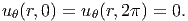
The boundary conditions that is of interest are also illustrated in figure 7.1. Thus, the cylinder is held fixed at constant length. Consequently, there is no axial displacement of the planes defined by z = 0 and z = L of the cylinder,
 | (7.58) |
where uz represents the axial component of the displacement field. Then, the outer surface defined by r = ro, of the cylinder is traction free, i.e.,
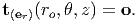 | (7.59) |
On the remaining surface, the inner surface defined by r = ri, of the cylinder only radial stress acts as shown in figure 7.1. Therefore,
 | (7.60) |
where pi is some positive constant. By virtue of the boundary conditions being independent of time and the constitutive relation is that of an elastic2 response, we are justified in assuming that the body is in static equilibrium under the action of boundary traction and hence a = o. Strictly, the traction boundary condition has to be applied on the deformed surface and not on the original surface. However, as discussed in section 7.2, we approximate the deformed surface with the original surface since they are close, in lieu of our assumptions that the magnitude of the displacement is small and that the magnitude of the components of the displacement gradient is also small.
To proceed further one has to decide whether to use displacement or stress as the basic unknown. Here we use displacement as the basic unknown. In general, one needs to solve the three partial differential equations involving the components of the displacement field, (7.22). Note by using (7.22) instead of (7.15), we have ignored the body forces and as per the discussion above we have assumed the body to be in static equilibrium.
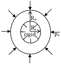
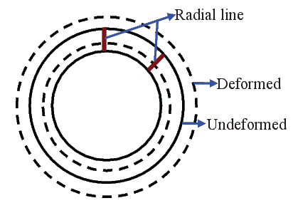
Next, in order to avoid solving partial differential equations, appropriate assumptions are made for the displacement field so that the governing equation (7.22) reduces to a ordinary differential equation. This is possible because, for mixed boundary condition boundary value problems for bodies in static equilibrium and in the absence of body forces, it is shown in section 7.5.1 that there exist a unique solution for a body made up of a material that obeys isotropic Hooke’s law. In light of the boundary condition (7.58) we assume uz = 0. Further, we expect the cross section of the cylinder to deform as shown in the figure 7.2. That is we expect the circular cross section to remain circular but with a different radius and initially straight radial lines on the cross section to remain straight after deformation. Further we assume that there is no axial variation in the displacement field, that is any section along the axis of the cylinder deforms in the same fashion. These suggest that there is no circumferential component of the displacement field, i.e., uθ = 0 and that the radial component of the displacement field vary radially only. Thus,
 | (7.61) |
Substituting equation (7.61) for displacement field in (7.22) and using equations (2.259), (2.260) and (2.261) we obtain
![[ 2 ]
(λ + 2μ) d-ur-+ dur1-- ur- = 0.
dr2 dr r r2](main882x.png) | (7.62) |
Since, (λ + 2μ) ≠ 0, for equation (7.62) to hold we require
 | (7.63) |
Solving the ordinary differential equation (7.63) we get
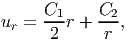 | (7.64) |
where C1 and C2 are integration constants to be found from the boundary conditions (7.59) and (7.60). Having found the unknown function in the displacement field (7.61), using (2.259) the cylindrical polar coordinate components of linearized strain can be computed as,
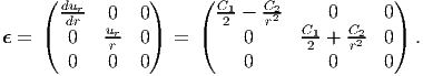 | (7.65) |
Substituting the above strain in the constitutive relation (7.2) the cylindrical polar coordinate components of the Cauchy stress is obtained as
 | (7.66) |
Recognizing that for the above state of stress, t(er) = [(λ + μ)C1 - μC2∕r2]e r, boundary conditions (7.59) and (7.60) yield
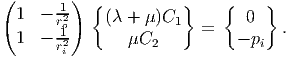 | (7.67) |
Solving the above equations we obtain:
 | (7.68) |
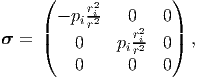
Substituting equation (7.68) in (7.66),
![( )
---r2i-- [ r2o]
| pi(r2o-r2i) 1 - r2 0[ ] 0 |
σ = || 0 p --r2i-- 1 + r2o 0 || ,
( i(r2o-r2i) r2 2 )
0 0 2νpi--r2i-2
(ro-ri)](main889x.png) | (7.69) |
where we have used (6.79) to deduce that 2ν = λ∕(λ + μ). Substituting equation (7.68) in (7.64),
![r2 [ r r2]
ur = pi--2-i-2-- --------+ -o- .
(ro - ri) (λ + μ ) rμ](main890x.png) | (7.70) |
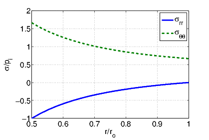
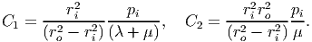
Figure 7.3 plots the variation of the radial (σrr) and hoop (σθθ) stresses with respect to r as given in equation (7.69) when ri = ro∕2. It is also clear from equation (7.69) that the axial stresses do not vary across the cross section. When ri = ro∕2, the constant axial stress value is 2piν∕3. Thus, we find that due to inflation of the annular cylinder, tensile hoop stresses develop and the radial stresses are always compressive. The magnitude of the hoop stress is greater than radial stress. The magnitude of the axial stress is nearly one-tenth of the maximum hoop stress and it is tensile when ν > 0 and compressive when ν < 0 and is zero when ν = 0. Next, we physically explain this variation of the axial stresses with the Poisson’s ratio. The hoop stresses by virtue of being tensile in nature will cause a reduction in the axial length due to Poisson’s effect3 if the Poisson’s ratio, ν > 0 and increase in length if ν < 0 and no change if ν = 0. Similarly, the radial stress being compressive in nature will cause an increase in the axial length when ν > 0, decrease in axial length when ν < 0 and no change in axial length when ν = 0. However, the actual change in axial length would be a sum of both the change in length due to hoop and radial stress. Since, the hoop stress is more than the radial stress, if no axial force is applied, the axial length would reduce when ν > 0, will not change when ν = 0 and will increase when ν < 0. Thus, if the length is to remain unchanged, a tensile axial force has to be applied to counter the reduction in length when ν > 0 and a compressive axial force when ν < 0 and no axial force is required when ν = 0. It can be seen from the expression for axial stress in equation (7.69) that the expression for the axial stresses is consistent with the expectation that it be positive when ν > 0, negative when ν < 0 and zero when ν = 0.
Now, we study the changes that occur to the thickness of the annular cylinder. Towards this, the ratio of change in thickness of the cylinder, Δt to its original thickness is obtained as
![Δt u (r ) - u (r) p r r2 { r [ r ] 1 - 2ν }
--- = --r-o-----r--i-= -i---o-------i--2- 1 - -o+ 1 - -i ------- ,
t ro - ri μ ro - ri(r2o - ri) ri ro (1 - ν)](main893x.png) | (7.71) |
where we have used (6.80) to write Lamè constants in terms of the Poisson’s ratio, ν and Young’s modulus E. Figure 7.4 plots the variation in the ratio of change in thickness of the cylinder to its original thickness as a function of the thickness of the cylinder for various possible values of Poisson’s ratio for a given radial component of the normal stress at the inner surface, pi. It can be seen from the figure that while the thickness decreases when ν ≥ 0, thickness increases when ν < 0 for thickness less than a critical value. By virtue of the radial component of the normal stress being compressive in nature one would expect a reduction in the thickness of the cylinder. However, the hoop stress being in tension, due to Poisson’s effect there would be reduction in thickness when ν > 0 and an increase when ν < 0. The actual change in the thickness is the sum of both the reduction due to radial stress and alteration due to hoop stress. Hence, the thickness decreases when ν ≥ 0 and increases when ν < 0 for thickness less than a critical value.
Finally, we would like to show that due to inflation the inner as well as outer radius of the cylinder increases. Noting that the deformed inner radius of the cylinder is ri + ur(ri) and that of the deformed outer radius is ro + ur(ro), for these radius to increase we need to show that ur(ri) > 0 and ur(ro) > 0. Towards this, using equation (7.70) and (6.80) we obtain,
![2 [ 2]
ur(r) = rpi ---ri---- (1---2ν)-+ ro .
μ (r2o - r2i) (1 - ν) r2](main894x.png) | (7.72) |
Recollecting from table 6.1, that the physically possible values for the Poisson’s ratio is: -1 < ν ≤ 0.5, it is straightforward to see that (1 - 2ν)∕(1 - ν) ≥ 0 for these possible range of values for ν. Also, it can be seen from table 6.1 that μ > 0. Further, by definition ro > ri and pi > 0. Therefore, ur(r) > 0 for any r, since each term in the expression for ur is positive. Hence, in particular ur(ri) > 0 and ur(ro) > 0 and hence the radius of the cylinder increases due to inflation, as one would expect.
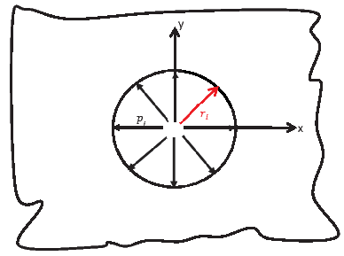
As a limiting case of the above solution, we would like to study the problem of
a hole subjected to uniform radial component of the normal stress in an
infinite medium as shown in figure 7.5. We continue to use cylindrical
polar coordinates. Therefore the body in the reference configuration is
assumed to occupy the region of the Euclidean point space defined by =
{(r,θ,z)|ri ≤ r < ∞, 0 ≤ θ ≤ 2π,-∞ < z < ∞}. The boundary conditions for
this problem is essentially same as that in the inflation of an annular cylinder,
except that now ro tends to ∞. For completeness the boundary conditions for the
present problem is:
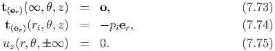
 | (7.76) |
 | (7.77) |
Thus, we find that both the stress and the displacement tend to zero as r tends to ∞. This means that the effect of pressurized hole is not felt at a distance far away from the hole.
Having studied the problem of pressurized hole, in the following section we shall study the influence of the hole to uniaxial tensile load applied to the infinite medium with the hole.
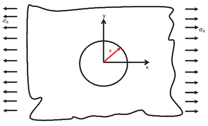
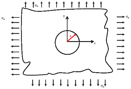
In the second boundary value problem that we study, the body is an infinite
medium with a circular stress free hole subjected to a far field tension along the
x-direction as shown in the figure 7.6. We envisage to solve this boundary value
problem using the stress formulation. In particular we assume plane stress state
and the body to be two dimensional and use cylindrical polar coordinates
to study this problem. Thus, the body in the reference configuration is
assumed to occupy a region in the Euclidean point space defined by =
{(r,θ)|a ≤ r < ∞, 0 ≤ θ ≤ 2π}, where a is a constant characterizing the size of
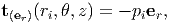
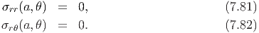
the hole in the infinite medium. The boundary conditions that is of interest are
 | (7.83) |
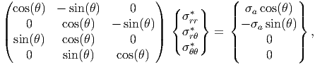
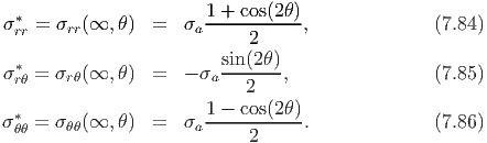
where σij* represents the value of the stress at (∞,θ). Of the four equations only 3 are independent. Picking any three equations and solving for the cylindrical polar components of the stress, we obtain
Thus, the boundary conditions translate into five conditions on the components of the stress given by equations, (7.81), (7.82), (7.84), (7.85) and (7.86).Based on the observation that the far field stresses are a function of cos(2θ), we infer that the Airy’s stress function, ϕ also should contain cos(2θ) term. Then, since the solution at θ equal to 0 and 2π should be the same, the Airy’s stress function can depend on θ only through the trigonometric functions present in the general solution (7.57). We assume Airy’s stress function with only five constants from the general solution (7.57) as,
![ϕ = a ln(r) + a r2 + [a r2 + a r-2 + a ]cos(2θ),
02 03 21 23 24](main904x.png) | (7.87) |
and examine whether the prescribed boundary conditions can be met. Consideration that the stress at ∞ be finite required dropping of the terms r2 ln(r) and r4. The constant a 01 does not enter the expressions for stress and hence indeterminate. So we assumed it to be zero. For the assumption of Airy’s stress function (7.87), the cylindrical polar components of the stress is computed using (7.53) to be
Now, the boundary conditions: (7.81), (7.82) and (7.84) yield:
 | (7.91) |
where we have equated the coefficients of cos(2θ), sin(2θ) and the constant to the values of the right hand side of these equations. It can be seen that the equations (7.85) and (7.86) yield the same last two equations in (7.91). Solving the linear equations (7.91) for aij’s, we obtain
 | (7.92) |
Since, we are able to meet the required boundary conditions with the assumed form of the Airy’s stress function, this is the required stress function.
Substituting the constants (7.92) in the equations (7.88) through (7.90) we obtain
Having obtained the stress, we compute the strains from these stresses using the constitutive relation (7.54) as Integrating equation (7.96) we obtain,![{ [ 2 [ 4] ] 2 }
ur = σa- (1 --ν)r + (1-+-ν) a--+ r - a-- cos(2θ) + -4 a-cos(2θ)
2 E E r r3 E r
df
+ --,
dθ](main910x.png) | (7.99) |
 (θ) is a function of θ. Substituting (7.99) in equation (7.97) and
integrating we find
(θ) is a function of θ. Substituting (7.99) in equation (7.97) and
integrating we find
![σa { (1 + ν) [ a4] (1 - ν )a2}
u θ = ---- ------- r + -3- + 2 ---------- sin(2θ) + f(θ) + g(r),
2 E r E r](main912x.png) | (7.100) |
where g(r) is some function of r. Substituting equations (7.99) and (7.100) in equation (7.98) and simplifying we obtain
 | (7.101) |
Since g is a function of only r and f only of θ, we require
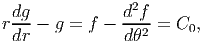 | (7.102) |
where C0 is a constant. Solving the linear ordinary differential equations (7.102) we obtain
 | (7.103) |
where Ci’s are constants. To ensure that the tangential displacement of the ray θ = 0 and θ = 2π to be the same and there be no rigid body displacement we require that,
 | (7.104) |
The condition (7.104) translates into requiring C1 = C2 = C3 = 0. Thus, the displacement field is computed to be,
![σa { (1 - ν) (1 + ν) [a2 [ a4] ] 4 a2 }
ur = --- -------r + ------- ---+ r - -3-cos(2θ ) + -----cos(2 θ) ,
2 E E r r E r
(7.105)
σ { (1 + ν)[ a4] (1 - ν) a2}
u θ = - -a- ------- r + -3- + 2------- --- sin(2θ). (7.106)
2 E r E r](main917x.png)
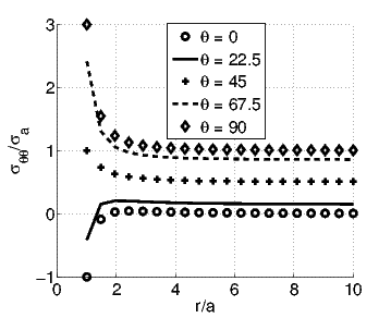
First we begin with hoop stress, σθθ given in equation (7.94). Recollecting that
the extremum value of a function could occur either at the boundary points or at
points where the derivative of the function goes to zero, the extremum hoop stress
could occur at a radial location, r = a , when cos(2θ) > 0 or at the
boundary points, r = a and r tending to ∞. In figure 7.7 we plot the
hoop stress as a function of r for various values of θ. As expected, the
function is monotonically decreasing function of r when cos(2θ) < 0 and
therefore the maximum value occurs at r = a for this case. When cos(2θ) >
0, the minimum occurs at r = a, then the maximum occurs when r =
a
, when cos(2θ) > 0 or at the
boundary points, r = a and r tending to ∞. In figure 7.7 we plot the
hoop stress as a function of r for various values of θ. As expected, the
function is monotonically decreasing function of r when cos(2θ) < 0 and
therefore the maximum value occurs at r = a for this case. When cos(2θ) >
0, the minimum occurs at r = a, then the maximum occurs when r =
a and then the stress decreases and asymptotically reaches
the value of σa[1 - cos(2θ)]∕2. Therefore, at r = a an extremum of the
hoop stress occurs. The circumferential variation of the hoop stress at
r = a is given by σa[1 - 2 cos(2θ)]. Hence, the maximum hoop stress
occurs at r = a and θ = π∕2 (or θ = 3π∕2) and the value of the maximum
hoop stress is 3σa. Thus, the stress concentration factor, defined as the
ratio of the maximum stress in the structure to the far field stress is 3 (=
σθθmax∕σ
a).
and then the stress decreases and asymptotically reaches
the value of σa[1 - cos(2θ)]∕2. Therefore, at r = a an extremum of the
hoop stress occurs. The circumferential variation of the hoop stress at
r = a is given by σa[1 - 2 cos(2θ)]. Hence, the maximum hoop stress
occurs at r = a and θ = π∕2 (or θ = 3π∕2) and the value of the maximum
hoop stress is 3σa. Thus, the stress concentration factor, defined as the
ratio of the maximum stress in the structure to the far field stress is 3 (=
σθθmax∕σ
a).
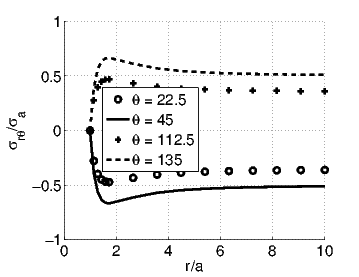
Next, we study the circumferential shearing stress, σrθ given in equation
(7.95). The extremum value of this stress occurs at a radial location r = a and
the value of the circumferential shearing stress at this radial location is
-2σa sin(2θ)∕3. At the boundary points the circumferential shearing stress takes
values 0 at r = a and -σa sin(2θ)∕2. The variation of σrθ with the radial location,
r and the orientation of the ray, θ is shown in figure 7.8. Thus, it can be seen that
the absolute maximum value of the stress, σrθ occurs at r = a
and
the value of the circumferential shearing stress at this radial location is
-2σa sin(2θ)∕3. At the boundary points the circumferential shearing stress takes
values 0 at r = a and -σa sin(2θ)∕2. The variation of σrθ with the radial location,
r and the orientation of the ray, θ is shown in figure 7.8. Thus, it can be seen that
the absolute maximum value of the stress, σrθ occurs at r = a , θ = mπ∕4,
where m takes one of the values from the set {1, 3, 5, 7} and this maximum value
is 2σa∕3.
, θ = mπ∕4,
where m takes one of the values from the set {1, 3, 5, 7} and this maximum value
is 2σa∕3.
 (a) When r varies between 1 and 10
 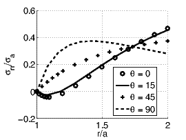 (b) When r varies between 1 and 2
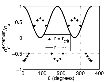
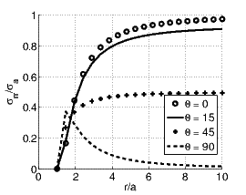
Finally, we examine the radial stress, σrr given in equation (7.93). An extremum value of this stress occurs at
![∘ ------------------------
rcrit = a 6cos(2θ)∕[1 + 4cos(2θ)]](main927x.png) | (7.107) |
when4
0 ≤ θ ≤ π∕6 or 2π∕6 ≤ θ ≤ 4π∕6 or 5π∕6 ≤ θ ≤ 7π∕6 or 8π∕6 ≤ θ ≤
10π∕6 or 11π∕6 ≤ θ ≤ 2π. This extremum value of the radial stress is
-σa{11 cos(2θ)∕9 + 1∕9 + 5∕[36 cos(2θ)]}∕2. At the boundary the radial stresses
takes the value 0 at r = a and σa[1 + cos(2θ)]∕2 as r tends to ∞. Figure 7.9
portrays the variation of the radial stress with radial location, r for various
orientations of the ray, θ. It can be seen from the figure that for certain
orientations (say, θ = 90 degrees) the maximum value of the radial stress occurs
at r = a![∘ ------------------------
6cos(2θ)∕[1 + 4cos(2θ)]](main929x.png) and for some other orientations (say, θ = 15
degrees) the maximum value occurs when r tends to ∞. To understand
this, in figure 7.10 we plot the two extremum radial stresses - one at r
= rcrit and the other value that occurs when r tends to ∞. It can be
seen from the figure that when π∕3 ≤ θ ≤ 2π∕3 and 8π∕3 ≤ θ ≤ 10π∕3
the maximum radial stress occurs at rcrit and for all other values of θ it
occurs as r tends to ∞. In any case the maximum value is always less than
σa.
and for some other orientations (say, θ = 15
degrees) the maximum value occurs when r tends to ∞. To understand
this, in figure 7.10 we plot the two extremum radial stresses - one at r
= rcrit and the other value that occurs when r tends to ∞. It can be
seen from the figure that when π∕3 ≤ θ ≤ 2π∕3 and 8π∕3 ≤ θ ≤ 10π∕3
the maximum radial stress occurs at rcrit and for all other values of θ it
occurs as r tends to ∞. In any case the maximum value is always less than
σa.
This concludes our illustration of the two techniques to solve boundary value problems in this chapter. However, in the remaining chapters we shall see employment of these techniques to solve more boundary value problems of interest in engineering.
In this section, we record two results that are useful while solving boundary value problems. One result tells when one can expect an unique solution to a given boundary value problem. The other allows us to construct solutions to complex boundary conditions from simple cases.
Now, we are interested in showing that there could at most be one solution that could satisfy the prescribed displacement or mixed boundary conditions, in a given body made of a material that obeys Hooke’s law and in static equilibrium with no body forces acting on it. If traction boundary condition is specified, we shall see that the stress is uniquely determined but the displacement is not for the bodies made of a material that obeys Hooke’s law and in static equilibrium with no body forces acting on it.
Towards this, we consider a general setting with being some region occupied
by the body and ∂ the boundary of the body. Let us also assume that
displacement is prescribed over some part of the boundary ∂u and traction
specified on the remaining part of the boundary, ∂σ. Let (u1, σ1) and (u2, σ2)
be the two distinct solutions to a given boundary value problem. Let us
define
 | (7.108) |
By virtue of (u1,σ1) and (u2, σ2) satisfying the specified boundary conditions,
First, we examine the term,
 | (7.111) |
here to obtain the last equality we have used (2.104) and the fact that the Cauchy stress σ is a symmetric tensor. Since, we are interested in materials that obey isotropic Hooke’s law, we substitute for the stress from5
![[ ]
σ = K - 2-G tr(ϵ)1 + 2G ϵ,
3](main933x.png) | (7.112) |
in (7.111) to obtain
![{ }
W = K [tr(ϵ)]2 + 2G tr(ϵ2) - 1[tr(ϵ)]2 .
3](main934x.png) | (7.113) |
As recorded in table 6.1 G > 0 and K > 0. Further recognizing that irrespective of the sign of the Cartesian components of the strain,
![1
tr(ϵ2) ---[tr(ϵ)]2
3
= 1[(ϵxx - ϵyy)2 + (ϵyy - ϵzz)2 + (ϵzz - ϵxx)2] + 2ϵ2 + 2ϵ2 + 2ϵ2 > 0,
3 xy yz xz](main935x.png) | (7.114) |
 | (7.115) |
as long as ϵ ≠ 0.
Next, we want to express
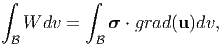 | (7.116) |
in terms of the boundary conditions alone. Towards this, using the result in equation (2.219) we write
 | (7.117) |
Since the body is in static equilibrium and has no body forces acting on it, from equation (7.6) div(σ) = o. Using div(σ) = o in equation (7.117) and substituting the result in (7.116) we get
 | (7.118) |
where to obtain the last equality we have used the result (2.267). Substituting the conditions (7.109) and (7.110) on the displacement and stress, in (7.118) that
 | (7.119) |
Since, from equation (7.115) the integrand in the equation (7.119) is positive and W = 0 only if ϵ = 0, it follows that ϵ = 0 everywhere in the body. Then, it is straight forward to see that σ = 0, everywhere in the body. It can then be shown that, we do this next for a special case, the conditions ϵ = 0 everywhere in the body and (7.109) imply u = o everywhere in the body.
Integrating the first order differential equations on the Cartesian components of the displacement field when ϵ = 0, we obtain
 | (7.120) |
where Ki’s are constants. Knowing the displacement of 3 points, say (x1,y1,z1), (x2,y2,z2) and (x3,y3,z3), that are not collinear to be zero, the constants Ki’s could be uniquely determined by solving the following system of equations:
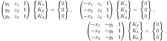 | (7.121) |
Hence, we conclude that the solution to the boundary value problem involving a body in static equilibrium, under the absence of body forces and made of a material that obeys isotropic Hooke’s law is unique except in cases where only traction boundary condition is specified. As a consequence of this theorem, if a solution has been found for a given boundary conditions it is the solution for a body in static equilibrium, under the absence of body forces and made of a material that obeys isotropic Hooke’s law.
This principle states that For a given body made up of a material that obeys isotropic Hooke’s law, in static equilibrium and whose magnitude of displacement is small, if {u(1),σ(1)} is a solution to the prescribed body forces, b(1) and boundary conditions, {ub(1),t (n)(1)} and {u(2),σ(2)} is a solution to the prescribed body forces, b(2) and boundary conditions, {u b(2),t (n)(2)} then {u(1) + u(2),σ(1) + σ(2)} will be a solution to the problem with body forces, b(1) + b(2) and boundary conditions, {u b(1) + u b(2),t (n)(1) + t (n)(2)}
The proof of the above statement follows immediately from the fact that equation (7.23) is linear. That is,
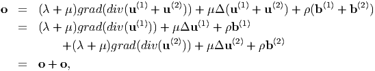
This is one of the most often used principles to solve problems in engineering. We shall illustrate the use of this principle in chapter 11.
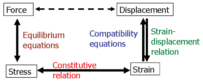
In this chapter, we formulated the boundary value problem for an isotropic material undergoing small elastic deformations obeying Hooke’s law. Two techniques were outlined to solve this problem. These two techniques are summarized in figure 7.11. Thus, in the displacement approach, one starts with the displacement use the strain displacement relation to compute the strain and then the constitutive relation to find the stress and finally use the equilibrium equations to get the governing equation that the displacement field has to satisfy along with the prescribed boundary conditions. In the stress approach, stress field is assumed in terms of a potential, such that equilibrium equations hold, then the strain is computed using the constitutive relation. In order to be able to obtain a smooth displacement field using this strain field, it is required that the stress potential satisfy the compatibility conditions along with the prescribed boundary conditions. We then illustrated these techniques by solving two boundary value problems, that of inflation of an annular cylinder and that of a plate with a hole subjected to uniaxial tension far away from the hole.
= {(r,θ,z)|Ri ≤ r ≤
(Ri + Ro)∕2, 0 ≤ θ ≤ 2π, 0 ≤ z ≤ H} and steel cylinder occupies
the region = {(r,θ,z)|(Ri + Ro)∕2 ≤ r ≤ Ro, 0 ≤ θ ≤ 2π, 0 ≤
z ≤ H}.
= {(r,θ,z)|Ri ≤ r ≤ (Ri +
Ro)∕2, 0 ≤ θ ≤ 2π, 0 ≤ z ≤ H} and aluminium cylinder occupies
the region = {(r,θ,z)|(Ri + Ro)∕2 ≤ r ≤ Ro, 0 ≤ θ ≤ 2π, 0 ≤
z ≤ H}.Take Young’s modulus of steel and aluminium to be Esteel = 200 GPa and Ealuminium = 70 GPa respectively and Poisson’s ratio of these materials to be νsteel = 0.3 and νaluminium = 0.27.
=
{(r,θ,z)|Ri ≤ r ≤ (δ + (Ri + Ro)∕2), 0 ≤ θ ≤ 2π, 0 ≤ z ≤ H} in the stress
free state is shrunk and fitted into a steel annular cylinder occupying the
region = {(r,θ,z)|(Ri + Ro)∕2 ≤ r ≤ Ro, 0 ≤ θ ≤ 2π, 0 ≤ z ≤ H} in the
stress free state. Then this composite shrink fitted cylinder is pressurized as
shown in figure 7.14. For this case solve parts (a) to (d) in problem 3.
Assume δ = 0.0001Ro. Take Young’s modulus of steel and aluminium to
be Esteel = 200 GPa and Ealuminium = 70 GPa respectively and
Poisson’s ratio of these materials to be νsteel = 0.3 and νaluminium =
0.27.![σ = λtr(ϵ)1 + 2μϵ, (7.2)
E [ ν ]
σ = ------- --------tr(ϵ)1 + ϵ , (7.3)
(1 + ν) (1 - 2ν)
(1 +-ν) ν-
ϵ = E σ - E tr(σ )1, (7.4)](main836x.png)
![div(λdiv(u )1) = grad (λdiv(u)),[ (]7.17)
div(2μ ϵ) = 2ϵgrad (μ) + μ div (grad(u)) + div((grad(u ))t) ,
(7.18)](main845x.png)
![[ 2 2 ] [ 2 2 ] 2
(1 - ν) ∂-σxx-+ ∂-σyy- - ν ∂-σzz-+ ∂-σzz- = 2(1 + ν) ∂-σxy, (7.24)
∂y2 ∂x2 ∂x2 ∂y2 ∂x∂y
[∂2σ ∂2 σ ] [∂2σ ∂2σ ] ∂2σ
(1 - ν) ---yy-+ ----zz - ν ---xx-+ ---xx- = 2 (1 + ν )---yz, (7.25)
[ ∂z2 ∂y2 ] [ ∂y2 ∂z2 ] ∂y∂z
∂2σxx ∂2σzz ∂2σyy ∂2σyy ∂2σxz
(1 - ν) ----2-+ ---2-- - ν ----2-+ ---2-- = 2 (1 + ν )-----, (7.26)
∂(z ∂x ∂x) ∂z ∂x∂z
-∂- ∂-σxy ∂σyz- ∂σxz- -∂2---
2(1 + ν)∂y ∂z + ∂x - ∂y = ∂z ∂x (σyy - ν [σxx + σzz]), (7.27)
( ) 2
2(1 + ν)-∂- ∂-σyz+ ∂σxz-- ∂-σxy = -∂----(σ - ν [σ + σ ]), (7.28)
∂z ∂x ∂y ∂z ∂x ∂y zz xx yy
∂ ( ∂ σ ∂σ ∂σ ) ∂2
2(1 + ν)--- ---xy + ---xz- --yz- = ----- (σxx - ν[σyy + σzz]), (7.29)
∂x ∂z ∂y ∂x ∂y ∂z](main851x.png)
![[ 4 4 4 2 2 ] 2 [ 2 2 ]
(1---2-ν)- ∂-ϕ-+ --∂-ϕ-- + ∂-ϕ-+ ∂-β- + ∂-β- = -∂-- ∂-ϕ-+ ∂--ϕ ,(7.35)
(ν - 1) ∂x4 ∂x2 ∂y2 ∂y4 ∂x2 ∂y2 ∂z2 ∂x2 ∂y2
(1 - 2 ν)[ ∂4ϕ ∂4ϕ ∂4 ϕ ∂2β ∂2β ] ∂2 [ ∂2ϕ ∂2 ϕ]
--------- --4-+ ---2--2 + ---4 + ---2 + ---2 = ---2 --2-+ ---2 ,(7.36)
(ν - 1) [ ∂y ∂y ∂z ∂z ∂y ∂z ] ∂x [ ∂y ∂z ]
(1 - 2 ν) ∂4ϕ ∂4ϕ ∂4 ϕ ∂2β ∂2β ∂2 ∂2ϕ ∂2 ϕ
(ν---1)-- ∂x4-+ ∂x2-∂z2 + -∂z4 + ∂x2- + ∂z2- = ∂y2- ∂x2-+ -∂z2 ,(7.37)](main857x.png)
![2 [ 2 { 2 2 } ]
-∂---- 2∂-ϕ-+ (1 - ν ) ∂-ϕ-+ ∂-ϕ- + (1 - 2ν)β = 0, (7.38)
∂x∂z ∂y2 ∂x2 ∂z2
∂2 [ ∂2ϕ { ∂2ϕ ∂2ϕ} ]
------ 2----+ (1 - ν ) ----+ ---- + (1 - 2ν)β = 0, (7.39)
∂x∂y [ ∂z2 { ∂x2 ∂y2 } ]
∂2 ∂2 ϕ ∂2ϕ ∂2ϕ
----- 2---2 + (1 - ν) ---2 + ---2 + (1 - 2ν)β = 0. (7.40)
∂y ∂z ∂x ∂y ∂z](main858x.png)
![∂4ϕ- ∂4ϕ- --∂4ϕ--
∂y4 + ∂x4 + 2∂x2 ∂y2 = 0, (7.44)
2 [ 2 2 ]
-∂-- ∂-ϕ-+ ∂-ϕ- = 0, (7.45)
∂y2 ∂x2 ∂y2
2 [ 2 2 ]
-∂-- ∂-ϕ-+ ∂-ϕ- = 0, (7.46)
∂x2 ∂x2 ∂y2
∂2 [ ∂2ϕ ∂2ϕ]
------ --2-+ --2- = 0, (7.47)
∂x∂y ∂x ∂y](main864x.png)
![t(er)(a,θ) = o, (7.78)
t(cos(θ)er- sin(θ)eθ)(∞, θ) = σa[cos(θ)er - sin(θ)eθ], (7.79)
t(sin(θ)er+cos(θ)eθ)(∞, θ) = o, (7.80)](main900x.png)
![[ ]
a02 6a23- 4a24-
σrr = r2 + 2a03 - 2a21 + r4 + r2 cos(2θ), (7.88)
[ ]
σθθ = - a02 + 2a03 + 2a21 + 6a23- cos(2θ), (7.89)
r2 r4
[ 6a 2a ]
σrθ = 2a21 - ---243- --224- sin(2θ), (7.90)
r r](main905x.png)
![σ {[ a2] [ a4 a2] }
σrr = -a- 1 - -2- + 1 + 3--4 - 4-2- cos(2θ) , (7.93)
2 {[ r ] [ r ] r }
σa a2 a4
σθθ = --- 1 + -2- - 1 + 3--4 cos(2θ) , (7.94)
2 [ r ] r
σa- a4- a2-
σrθ = - 2 1 - 3r4 + 2r2 sin(2θ). (7.95)](main908x.png)
![∂u
ϵrr = ---r
∂r{ [ [ ] ] }
σa- (1---ν) (1-+-ν) a2- a4- -4 a2-
= 2 E + E - r2 + 1 + 3r4 cos(2θ) - E r2 cos(2θ) ,
(7.96 )
1-∂uθ- ur-
ϵθθ = r ∂ θ + r
σ { (1 - ν) (1 + ν) [a2 [ a4] ] 4νa2 }
= --a ------- + ------- ---- 1 + 3 ---cos(2θ ) + -----cos(2θ) ,
2 E E r2 r4 E r2
(7.97 )
[ ]
ϵrθ = 1- 1-∂ur-+ ∂uθ-- u-θ
2 r ∂θ ∂r r
(1 + ν)σa [ a4 a2]
= - ---------- 1 - 3 -4 + 2-2- sin (2θ). (7.98 )
E 2 r r](main909x.png)