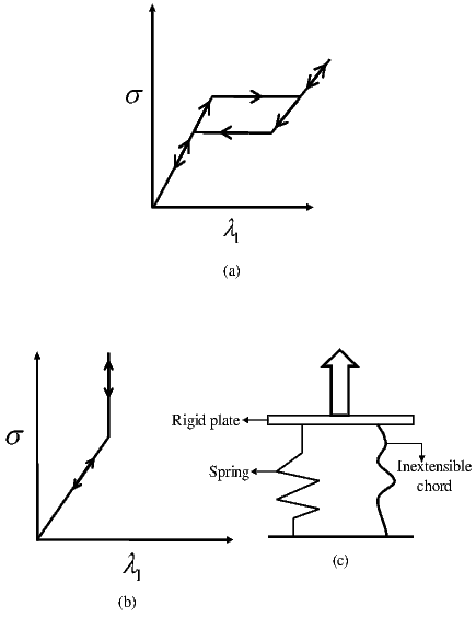
Figure 6.1: Uniaxial stress, σ versus axial stretch ratio, λ1 plot for (a)
superelastic process (b) mechanical model shown in (c).
The concepts and equations introduced in chapters 3 to 5, within the framework of non-relativistic mechanics, are essential to characterize kinematics, stresses and balance principles and as mentioned already these concepts and equations hold for any body undergoing a purely mechanical process. However, they do not distinguish one material from another which is contradictory with the experiments. Also, for a non-polar body while there are only seven equations1 there are thirteen2 scalar fields that needs to be determined. Thus, there are more unknowns in the balance laws than available equations and hence all of the unknown fields cannot be determined from the balance laws alone. In other words, balance laws alone are incapable of determining the response (displacement of the body due to an applied force) of deformable bodies3 . They must be augmented by additional equations, called constitutive relations or equations of state, which depends on the material that the body is made up of. A constitutive relation approximates the observed physical behavior of a material under specific conditions of interest. To summarize, constitutive relations are required for two reasons:
Thus, we may constitutively prescribe the six independent components of Cauchy stress. Now, for a non-polar body, we have as many equations as there are variables. Then, the balance of mass is used to obtain the density and balance of linear momentum to obtain the body force. By prescribing the constitutive relation only for the six components of the stress field, we have already made use of the balance of angular momentum as applicable for a non-polar body. We hasten to emphasize the arbitrariness in the choice of variables that are constitutively prescribed and those that are found from the balance laws.
Quantities characterizing a system at a certain time are called state variables. The state variables are quantities like stress, density. Contrary to some presentations of thermodynamics, we do not consider kinematical quantities as state variables. We treat them as independent variables, because they are the directly measurable quantities in an experiment. On the other hand, none of the state variables can be measured directly in an experiment. However, we require the state variables to depend (explicitly or implicitly) on the kinematical quantities and the function that establishes this relation between kinematic variables and state variables is called constitutive relation. Reemphasizing, these constitutive relation depend on the material that the body is made up of and of course, the process that is being studied.
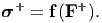
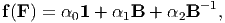
Naturally, it is at this stage where the major subdivisions of the subject, such as the theories of viscous flow, elasticity branch out. These subdivisions are nothing but assumptions made on which kinematic variables determine the Cauchy stress. For example, if Cauchy stress is assumed to be prescribed through a function of the Eulerian gradient of the velocity field, i.e., σ = g(grad(v)), then it can describe the flow of a viscous material. On the other hand, if Cauchy stress is assumed to be depend explicitly on the gradient of the deformation field, i.e., σ = f(F), then this can describe the elastic deformation of a solid. As this course is concerned about elastic response of the body, let us understand what we mean by elastic response?
All bodies deform under the application of load. Depending on the characteristics of this deformation, the process or the body is classified as elastic or inelastic. The characteristics of this deformation depends on the material, temperature, magnitude of the applied load and among many other factors. Now, let us understand the characteristics of a elastic process.
Some of the definitions of an elastic process in the literature are:
The first two definitions are popular in the literature. However, they are of little use because they cannot tell whether a process that the body is currently being subjected to is elastic. Such a conclusion can be arrived at only after subjecting the body to a complementary process. However, the last definition does not have such a drawback.
Further, it turns out that these various definitions are not equivalent. To see this, consider the uniaxial stress versus stretch ratio plot shown in figure 6.1a. Such a response, possible in shape memory alloys, would qualify as elastic only if the first definition is used. Since, the stress corresponding to a given stretch ratio depends on whether it is being loaded or unloaded it is not elastic according to the second definition. Also, since the loading and unloading path are different, there will be dissipation (wherein the mechanical energy is converted into thermal energy). Hence, it cannot be elastic by the last definition either.
Consider a axial stress vs. stretch response as shown in figure 6.1b which will be characterized as elastic according to definitions one and three. But the value of state variable stress could be anything corresponding to a stretch ratio of Λo. Hence, it is not elastic according to definition two. Of course, such a stress versus stretch response occurs for an idealized system made of a spring and an inextensible chord as shown in figure 6.1c. But then elasticity is an idealized process too and biological soft tissues response can be idealized as shown in figure 6.1b.
For us, a process is elastic only if it is consistent with all three definitions.
Before proceeding further a few words of caution is necessary. In reality, no process is elastic but some are close to being elastic. It is common in the literature, as we also did in the first paragraph, to call a material or a body to be elastic. This is incorrect, in a strict sense. It is the process that the body is being subjected to which is elastic. After all, the same body under different circumstances deforms inelastically.
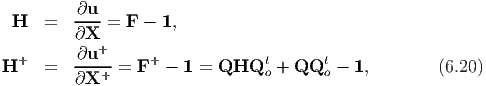
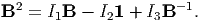
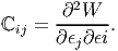
Based on the above definition of elasticity, it can be shown that the Cauchy stress, σ, in an elastic process would at most depend on the deformation gradient, F, three material unit vectors, Mi and the state of Cauchy stress in the reference configuration4 , σR and thus,
 | (6.1) |
In other words, equation (6.1) is an assumption on how the state variable, stress, varies with the motion of the body. Since, by definition 2 for an elastic process, the value of stress cannot depend on the history of the motion field that the body has experienced, we are assured that there is an implicit function that relates the Cauchy stress and the deformation gradient.
We shall assume σR = 0, that is the reference configuration is stress free and that the Cauchy stress is related explicitly to the deformation gradient, so that equation (6.1) could be simplified to,
 | (6.2) |
Further if we assume that the material is isotropic, that is the response of the material is same in all directions (see section 6.3.2 for more detailed discussion), the Cauchy stress would not depend on the three unit material vectors, Mi. For this case, the Cauchy stress depends explicitly only on the deformation gradient, i.e.,
 | (6.3) |
Thus, we have to find the relation between the six independent components of the stress tensor and the nine independent components of the deformation gradient. To find this relation in general through experimentation alone is daunting, as we illustrate now. Let us say the relation between the components of the Cauchy stress (σij) and deformation gradient (Fkl) is linear and of the form,
 | (6.4) |
where Cijkl is the components of a constant fourth order tensor and δkl is the Kronecher delta. Even for this case, we have to find 6*9 = 54 constants which means we require 54 independent measurements. This is too many. While for metals this relationship is linear for polymers it is nonlinear. It is easy to see that the number of constants required in case of nonlinear relationship would be much higher than the linear case. Hence, if there is some way by which we can reduce the number of unknown functions from 6 and the variables that it depends on from 9 in equation (6.3) it would be useful. It turns out that this is possible and this is what we shall see next.
There are certain restrictions, guidelines and principles that are common which the constitutive relations for different materials and under different conditions of interest, should satisfy. Thus, we require the constitutive relation to ensure that the value of the state variables for a given state of the body are independent of the placement of the body in the Euclidean space and to honor the coordinate transformation rules. There is also, the concept of material symmetry which to a large extent determines the variables in the constitutive relation. The following section is devoted towards understanding these concepts.
While the physical body was given a mathematical representation, we made two arbitrary choices regarding:
Since these choices are arbitrary, the state of the body cannot depend on these choices. (Clearly, a body subjected to a particular load cannot fail just because, the body is mapped on to a different region of Euclidean point space or a different set of basis vectors is used.) Hence, the constitutive relations that relate these state variables with the independent variables, i.e., kinematic variables, should also not depend to these choices.
The value of state variables variables have to be invariant with respect to the above choices because they mathematically describe the state of the body. We emphasize that the value of the state variables have to be invariant and not same. Thus, while the value of scalar valued state variables like density have to be the same, the components of tensor valued state variables like stress will change with the choice of the basis according to the transformation rules discussed in section 2.6. However, as pointed out in 2.6 just because the components of a tensor is different does not mean they are different tensors. Only, if the value of at least one of the certain scalar valued functions of the components of the tensor are different5 , the two tensors are said to be different.
In this section, we shall explore the restrictions that needs to be placed on the constitutive relations so that they remain invariant for the different equivalent mappings of the body on to the Euclidean point space. From a physical standpoint, the same restriction could be viewed as requiring the constitutive relation of the body be the same irrespective of where the body is. That is, say, the deflection of the beam to a given set of loads should remain the same whether it is tested in Chennai or Delhi or Washington or London.
It should be realized that in the different mappings of the body onto the Euclidean space, it is the point space that changes and not the vector space. If the vector space were to change, it means that we are changing the basis vectors. Further, it is assumed that the scale used to measure distances between two points does not change. Consequently, the distance between any two points in the body does not change due to these different mappings of the body. Hence, this restriction, as we shall see, tantamount to requiring that the state variables be invariant to superposed rigid body rotation of the current or the reference configuration.
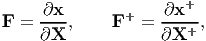
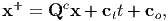
Let x and x+ denote the position vector of a material particle at time t, mapped on to different regions of the Euclidean point space. Then, they are related by the equation:
 | (6.5) |
where Q and c are functions of time, t and Q is an orthogonal tensor, not necessarily a proper orthogonal tensor6 . While it is easy to see that (6.5) preserves the distance between any two points, the converse can be proved by following the same steps as that outlined in section 3.10.1.
Since, similar non-uniqueness exist with respect to placers for the reference configuration
 | (6.6) |
where X and X+ are the position vectors of same material particle mapped on to the different regions of the Euclidean point space, Qo is a constant orthogonal tensor and co is a constant vector.
Next, we like to compute the standard kinematical quantities and see how they change due to these equivalent mappings of the body on to the Euclidean point space. This is a prerequisite to find the restrictions on the constitutive relations due to this requirement.
We begin by considering the transformations of the motion field, χ. Let
 | (6.7) |
then using equations (6.5) and (6.6) we obtain
 | (6.8) |
Now, we can find the relation between the deformation gradients, F and F+ defined as
 | (6.9) |
using (6.6), (6.8) and chain rule for differentiation to be
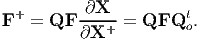 | (6.10) |
Next, we find the relation between the velocity fields, v and v+ defined as
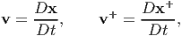 | (6.11) |
using equation (6.5) as
 | (6.12) |
Similarly, we obtain the relationship between accelerations a and a+ as
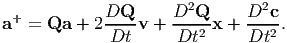 | (6.13) |
In order to simplify equations (6.12) and (6.13) we introduce, the skew tensor
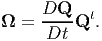 | (6.14) |
To show that Ω is a skew tensor, taking the total time derivative of the relation QQt = 1, we obtain
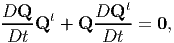 | (6.15) |
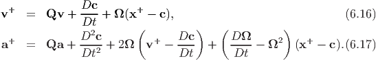
from which the required result follows. In lieu of definition (6.14), equations (6.12) and (6.13) can be written as
where we have made use of the identity
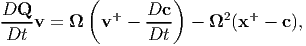 |
to obtain (6.17).
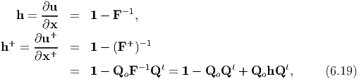
Now, we would like to see how the displacement transforms due to different placements of the body in the Euclidean point space. Recalling that the displacement field is defined as:
 | (6.18) |
The Eulerian displacement gradient transforms like
where we have used (6.10) and (3.34). Similarly, the Lagrangian displacement gradient, is computed to be using (6.10) and (3.33). It is apparent from the above equations that displacement gradient transforms as QhQt (or Q oHQot) only if Q = Qo.Then, it is straightforward to show that the right and left Cauchy-Green deformation tensor transform as:
 | (6.21) |
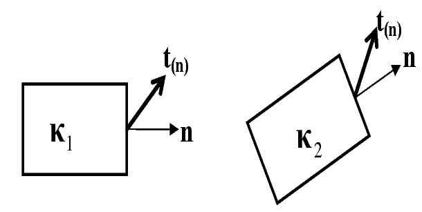
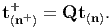
Next, we examine what happens to stress tensors due to different placements of the body in the current configuration. Recalling traction is related to the Cauchy stress, by the relation t(n) = σn, where n is the outward unit normal at a point x on the boundary surface ∂𝔅t of an arbitrary region 𝔅t.
As evidenced from the figure (6.2) a different placer of the body in the
Euclidean space, in general, alters the orientation of the normal with respect to a
fixed set of basis vectors. Let n and n+ denote the outward unit normals to the
same material surface ∂ and at the same material particle, P, in two different
placements of the body in the Euclidean space, 𝔅t and 𝔅t+. Since, we are
interested in the same material surface, we can appeal to Nanson’s formula (3.72)
to relate the unit normals as
and at the same material particle, P, in two different
placements of the body in the Euclidean space, 𝔅t and 𝔅t+. Since, we are
interested in the same material surface, we can appeal to Nanson’s formula (3.72)
to relate the unit normals as
 | (6.22) |
where we have made use of the equation (6.5) which provides the relationship between the placements 𝔅t and 𝔅t+.
Similarly, the traction vector t(n) and t(n+)+ acting on the same material
surface, ∂ and at the same material particle P, in two different placements of the
body, 𝔅t and 𝔅t+ are related through:
 | (6.23) |
To obtain the above equation we have made use of the fact that the normal and shear traction acting on a material surface in two different placements of the body in the current configuration has to be same, i.e., t(n+)+ ⋅ n+ = t (n) ⋅ n. Then, (6.23) is obtained by recognizing that (Qtt (n+)+ - t (n)) ⋅ n = 0 for any choice of n where we have made use of (6.22).
Since, t(n+)+ = σ+n+ and t (n) = σn, we obtain
 | (6.24) |
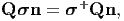
using equations (6.22) and (6.23) and the above equation has to hold for any choice of n. Therefore, the Cauchy stress will transform as
 | (6.25) |
Since, the definition of Cauchy stress is independent of the choice of reference configuration, different placers of the reference configuration, does not cause any change in the value of the Cauchy stress.
Next, let us see how body forces transform. These forces are essentially action at a distance forces acting along a straight line joining the material particles in the body under investigation to another point in space belonging to some other body. Thus, if r is the position vector of the point belonging to another body, then the direction along which b acts, is given by (x - r)∕(∣x - r∣). Then, in a different placement of the body the body force acts along a direction (x+ - r+)∕(∣x+ - r+∣). Because the new placement of the body is related to its original placement by equation (6.5), we obtain
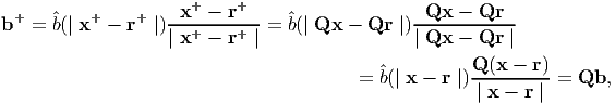 | (6.26) |
 (⋅) denotes a function of the distance between two points of interest.
Here r+ = Qr + c because the transformation rule is applicable not only to points
that the body under study occupies but to its neighboring bodies as well. This is
required so that the relationship between the body under investigation and its
neighbors are preserved.
(⋅) denotes a function of the distance between two points of interest.
Here r+ = Qr + c because the transformation rule is applicable not only to points
that the body under study occupies but to its neighboring bodies as well. This is
required so that the relationship between the body under investigation and its
neighbors are preserved.
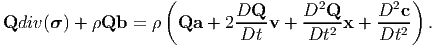
Finally, for future reference, div(σ) transforms due to equivalent placements of the body as,
 | (6.27) |
where div+ denotes the divergence with respect to x+.
Till now, we have just seen how various quantities transform between different placements of the same body in the same state. Using this we are in a position to state what restriction the requirement that the state variables be invariant to the different placers of the body in the same state places on the constitutive relation, given it depends on certain kinematic quantities and other state variables. For example, as we saw above for elastic process the stress is a function of deformation gradient, i.e.,
 | (6.28) |
Now, due to different placement of the body in the reference and current configurations,
 | (6.29) |
Note that the function does not change and this is what restricts the nature of the function. Using equations (6.25) and (6.10), (6.29) can be written as
 | (6.30) |
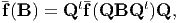
Substituting for σ from equation (6.28) we obtain a restriction of the form of the function f as:
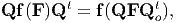 | (6.31) |
for any orthogonal tensors Q and Qo and F ∈ ⊆ Lin+, the set of all linear
transformations whose determinant is positive.
⊆ Lin+, the set of all linear
transformations whose determinant is positive.
The question on how to obtain the form of the function, given the restriction (6.31), is dealt in detail next. To understand how this restriction (6.31) fixes the form of the tensor-valued tensor function, let us look at a similar requirement on scalar-valued scalar function, g(x). Say the restriction on this scalar function is: g(m * x) = m * g(x), where m is some arbitrary constant. It then immediately tells that the function is a linear function, i.e., g(x) = a * x, where a is some constant. Similarly, it transpires that the restriction (6.31) requires,
 | (6.32) |
where αi =  i(J1,J2,J3),
![-1 1∕2
J1 = tr(B ), J2 = tr(B ), J3 = [det(B)] = det(F ),](main712x.png) | (6.33) |
are the invariants of B.
Now, we show how equation (6.32) is obtained from the restriction (6.31). Towards this, first we set Q = 1 to obtain,
 | (6.34) |
where we have made use of the polar decomposition theorem (2.116). Then, let us pick Qo = R, since R is also an orthogonal tensor. With this choice equation (6.34) yields
 | (6.35) |
The last equality arises because B = V2 and square-root theorem, (2.147)
ensures the existence of an unique V such that V =  . Next, we shall
again appeal to equation (6.31) but now we shall not set Q to be 1 to
obtain
. Next, we shall
again appeal to equation (6.31) but now we shall not set Q to be 1 to
obtain
 | (6.36) |
∀ Q ∈ . The above equation can be rewritten as
 | (6.37) |
∀ Q ∈.
Theorem 7.1: A symmetric second order tensor valued function defined over the space of symmetric second order tensors, satisfies (6.37) if and only if it has a representation
 | (6.38) |
where α0, α1, α2 are functions of principal invariants of B, Ii, i.e.,
 | (6.39) |
Proof: 7 Before proving the above theorem we prove the following theorem:
Theorem 7.2: Let α be a scalar function defined over the space of symmetric
positive definite second order tensors. Then α(QBQt) = α(B) ∀ Q ∈ if and
only if there exist a function α, defined on  + ×+ ×+, such that α(B) =
α(λ1,λ2,λ3), where α(λ1,λ2,λ3) is insensitive to permutations of λi and λ1, λ2, λ3
are the eigenvalues of B. Hence, α(B) =
+ ×+ ×+, such that α(B) =
α(λ1,λ2,λ3), where α(λ1,λ2,λ3) is insensitive to permutations of λi and λ1, λ2, λ3
are the eigenvalues of B. Hence, α(B) =  (I1,I2,I3).
Proof: 8 Writing B in the spectral form
 | (6.40) |
where bi’s are the ortho-normal eigenvectors of B and hence
 | (6.41) |
Since, α(QBQt) = α(B) ∀ Q ∈, α(B) must be independent of the orientation
of the principal directions of B and must depend on B only through its
eigenvalues, λ1, λ2, λ3.
Next, choose Q to be a rotation of π∕2 about b3 so that Qb1 = b2, Qb2 = -b1 and Qb3 = b3. Hence,
 | (6.42) |
from which we deduce that α(λ1,λ2,λ3) = α(λ2,λ1,λ3). In similar fashion it can be shown that α is insensitive to other permutations of λi’s.
Finally, recalling that the eigenvalues are the solutions of the characteristic equation
 | (6.43) |
in principal, λi’s can be expressed uniquely in terms of the principal invariants
and hence α(B) =  (I1,I2,I3).
The converse of the theorem 7.2 is proved easily from the property of trace and determinants. Hence, we have proved theorem 7.2.
Theorem 7.3: If f satisfies (6.37) then the eigenvalues of f(B) are functions of the principal invariants of B.
Proof: Let γ(B) be the eigenvalue of f(B). Then,
![det[f(B ) - γ(B )1] = 0.](main726x.png) | (6.44) |
The corresponding eigenvalue of f(QBQt) is γ(QBQt) and hence
![--
det[f(QBQt ) - γ(QBQt )1] = 0.](main727x.png) | (6.45) |
This can be written as
![-- t t
det[Q{ f(B) - γ(QBQ )1 }Q ] = 0,](main728x.png) | (6.46) |
by using (6.37) and the relation QQt = 1. Using the property of determinants the above equation reduces to
![--
det[f(B ) - γ (QBQt )1] = 0,](main729x.png) | (6.47) |
which has to hold for all Q ∈. Comparing (6.44) and (6.47)
 | (6.48) |
for all Q ∈, which by theorem 2.2 implies that γ(B) =  (I1,I2,I3)
Theorem 7.4: If σ = f(B) satisfies (6.37) then f(B) is coaxial with B, i.e., the principal directions of B and f(B) would be the same.
Proof: Consider an eigenvector b1 of B and define an orthogonal transformation Q by
 | (6.49) |
i.e. Q is a reflection on the plane normal to b1. Now, QBQt = B and hence, by (6.37), Qσ = σQ. We therefore have
 | (6.50) |
and we see that Q transforms the vector σb1 into its opposite. Since, the only vectors transformed by the reflection Q into their opposites are the multiples of b1, it follows that b1 is an eigenvector of σ. Similarly, it can be shown that every eigenvector of B is also an eigenvector of σ. Hence, f(B) is coaxial with B.
Now we prove theorem 7.1.
Clearly, if (6.38) along with (6.39) holds then (6.37) is satisfied and hence we have to prove only the converse.
It follows from theorem 7.3 and theorem 7.4 that f(B) is coaxial with B and its eigenvalues are functions of the principal invariants of B. Let λ1,λ2,λ3 and f1,f2,f3 be the eigenvalues of B and f(B) respectively and consider the equations
 | (6.51) |
for the three unknowns α0, α1, α2. Assuming the λi and fi are given and that λi’s are distinct it follows that αi’s are determined uniquely in terms of λi and fi which are themselves determined uniquely by the principal invariants of B. Thus, since B is coaxial with f(B) and αi are functions of the principal invariants of B; equation (6.38) follows from (6.51) provided the eigenvalues of B are distinct, of course. When the eigenvalues of B are not distinct α2 or α1 and α2 could be chosen arbitrarily, depending on whether the algebraic multiplicity of the eigenvalues is 2 or 3 respectively. However, this choice may cause some αi to become discontinuous even when f(B) remains continuous, Truesdell and Noll [8] and Serrin [5] provide example of such cases.
Finally, from Cayley-Hamilton theorem, (2.142) we obtain
 | (6.52) |
Then, observing that the principal invariants of the positive definite, B, are related bijectively to the invariants J1, J2 and J3, as defined in (6.33), we note that
 | (6.53) |
for i = (0, 1, 2). Substituting (6.52) and (6.53) in (6.38) we obtain
 | (6.54) |
Before concluding this section let us investigate a couple of issues. The first issue is whether the balance laws should also be invariant to different placements of the body in the same state. A straight forward calculation will show that balance of mass is invariant to different placements of the same body in the same state. However, balance of linear momentum and hence angular momentum are not. In fact, due to equivalent placements of the body, the balance of linear momentum equation transforms as
 | (6.55) |
But for the above equation to be consistent, it is required that
 | (6.56) |
since, div(σ) + ρb = ρa. The above equation holds only for placements for which
 = o and Q(t) = Qc, a constant. Thus, a school of thought requires the
constitutive relations describing the state variables to be invariant only for
placements of the body related as:
= o and Q(t) = Qc, a constant. Thus, a school of thought requires the
constitutive relations describing the state variables to be invariant only for
placements of the body related as:
 | (6.57) |
where Qc is a constant orthogonal tensor, c t and co are constant vectors. Equation (6.57) is called Galilean transformation.
The other school of thought, argues that equivalent placements of the body in a particular state is a thought experiment to obtain some restriction on the constitutive relations describing the state variables which is not applicable for balance laws. The rational behind their argument is that for a given body force, the balance laws will hold only for certain motions of the body9 . On the other hand, there are no such restrictions for the constitutive relations. Hence, there is no inconsistency if motions that are not admissible according to the balance law are used to find restrictions on the constitutive relations. We find merit in this school of thought.
The second issue is on the existence of unique placer for the reference configuration. Some researchers are of the opinion that the placer to the reference configuration has to be unique for agreement on the material symmetry of the body. In section 6.3.2, we show that the opinion of these researchers is incorrect.
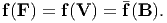
We have been writing equations in direct form, that is independent of the choice of basis vectors. To beginners it is natural to ask the question, if we were to continue to write equations in direct form what restriction can this choice of basis vectors place? To answer this question let us look at an example. Say, some person investigating the response of some body subjected to some process finds that Cauchy stress, σ is related to the deformation gradient, F, as σ = α(F - 1), where α is a constant. Even though we have written in direct notation, say, we change the basis vectors used to describe the reference configuration, then the matrix components of the Cauchy stress will not change. However, the matrix components of the deformation gradient will change resulting in a contradiction and inadmissability of the proposed relation.
To elaborate, recall that σ = σijei ⊗ ej and F = Fijei ⊗ Ej, where ei is the basis vectors used to represent the current configuration and Ej is the basis vectors used in the reference configuration. Then, let [] and [] represent the matrix components of the Cauchy stress and deformation gradient with respect to the {i} basis. Similarly, let [σ] and [F] denote the matrix components of the Cauchy stress and deformation gradient with respect to the {Ei} basis. It follows from the transformation laws 2.6 that
![[¯σ ] = [σ ], [F¯] = [F ][Q ],](main742x.png) | (6.58) |
where Qij = Ei ⋅j. Immediately, the contradiction in the constitutive relation, σ = α(F - 1) is apparent.
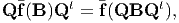
Let us see what restriction is placed on the form of the function (or functional) to ensure that it obeys the necessary transformation rules. Thus, say, we postulate that: σ = f(F). Let Qij = ei ⋅j and Qijo = E i ⋅j. Due to this transformation of the basis vectors in the current and the reference configuration, the stress transforms as [] = [Q]t[σ][Q] and the deformation gradient transforms as [] = [Q]t[F][Qo]. Then, we require that [] = [f([])]. Hence, the function f(⋅) should be such that
![t t o
[Q ][f([F ])][Q] = [f([Q ][F ][Q ])]](main743x.png) | (6.59) |
for any [Q] and [Qo] such that [Q][Q]t = [Q]t[Q] = [Qo][Qo]t = [Qo]t[Qo] = [1]
and for all F ∈⊆ Lin+.
While it is non-trivial to deduce the form of the function f(F) satisfying the condition (6.59), it is easy to verify that
 | (6.60) |
where B = FFt, α
i =  i(tr(B),tr(B-1), det(F)) upholds the condition
(6.59).
i(tr(B),tr(B-1), det(F)) upholds the condition
(6.59).
Looking at restriction (6.31) and (6.59) one might wonder on the need for (6.59). Because if (6.31) were to hold then (6.59) will always hold. However, recognize that (6.59) is a different requirement than (6.31) and these differences would be apparent for cases where the constitutive relation depends on velocity or its derivatives. To see this, a change of basis used to describe the current configuration results in the velocity vector transforming as [Q][v], which is different from (6.16) and hence the difference between the restrictions (6.59) and (6.31). To clarify, even if the basis were to change continuously with time, the velocity will transform as [Q(t)][v] because the choice of the basis determines only the components of the velocity vector and not the velocity of the particle which depends only on the relative motion of the particle and the observer.
Before looking at the concept of material symmetry, we have to understand what we mean by the body being homogeneous or inhomogeneous. Intuitively, we think that a body is homogeneous if it is made up of the same material. However, there is no particular variable in our formulation that uniquely characterizes the material and only the material. But the constitutive relation (or equation of state) which relates the state variables and the kinematic variable depends on the material. However, since the value of the kinematic variable, say the displacement or the deformation gradient, depends on the configuration used as reference, the constitutive relation also depends on the reference configuration or more particularly on the value of the state variables in the configuration used as reference. Hence, just because the constitutive relation for two particles are different does not mean that they are different materials, the difference can arise due to the use of different configurations being used as reference.
Consequently, mathematically, we say that two particles in a body belong to the same material, if there exist a configuration in which the density and temperature of these particles are same and with respect to which the constitutive equations are also same. In other words, what we are looking at is if the value of the state variables evolve in the same manner when two particles along with their neighborhood are subjected to identical motion fields from some reference configuration in which the value of the state variables are the same.
A body that is made up of particles that belong to the same material is called homogeneous. If a body is not homogeneous it is inhomogeneous. Now, say we have a body, in which different subsets of the body have the same constitutive relation only when different configurations are used as reference, i.e., any configuration that the body can take without breaking its integrity would result in different constitutive relations for different material particles, then the issue is how to classify such a body. Any body with residual stresses10 like shrink fitted shafts, biological bodies are a couple of examples of bodies that fall in this category. One school of thought is to classify these bodies also as inhomogeneous, we subscribe to this definition simply for mathematical convenience.
Having seen what a homogeneous body is we are now in a position to understand what an isotropic material is. Consider an experimentalist who has mathematically represented the reference configuration of a homogeneous body, i.e., identify the region of the Euclidean point space that this body occupies, has found the spatial variation of the state variables. Now, say without the knowledge of the experimentalist, this reference configuration of the body is deformed (or rotated). Then, the question is will this deformation (or rotation) be recognized by the experimentalist? Theoretically, if the experimentalist cannot identify the deformation (or rotation), then the functional form of the constitutive relations should be the same for this deformed and initial reference configuration. This set of indistinguishable deformation or rotation forms a group called the symmetry group and it depends on the material as well as the configuration that it is in. If the symmetry group contains all the elements in the orthogonal group11 then the material in that configuration is said to possess isotropic material symmetry. If the symmetry group does not contain all the elements in the orthogonal group, the material in that configuration is said to be anisotropic. There are various classes of anisotropy like transversely isotropic, orthorhombic, etc., depending on the elements contained in the symmetry group.
Here we like to emphasize on some subtleties. Firstly, we emphasize that the
symmetry group of a material depends on the configuration in which it is assessed.
Thus, the material in a stress free configuration could be isotropic but the same
material in uniaxially stressed state will not be isotropic. Secondly, we allow the
body to be deformed because it has been shown [10] that certain deformations
superposed on an uniaxially extended body does not alter the state of the body.
Hence, it should be recognized that the symmetry group,  ⊆
⊆ , the unimodular
group12 ,
since the volume cannot change in an equivalent placement of the body. In fact,
for a perfect gas the symmetry group, = . Thirdly, unlike in the restriction
due to objectivity, in this case only the body is rotated or deformed virtually, not
its surroundings. Even though like in the restriction due to objectivity the
rotation or deformation is virtual, it has to maintain the integrity of the body and
satisfy the balance laws, i.e., be statically admissible because the rotated or
deformed configuration is also in equilibrium.
, the unimodular
group12 ,
since the volume cannot change in an equivalent placement of the body. In fact,
for a perfect gas the symmetry group, = . Thirdly, unlike in the restriction
due to objectivity, in this case only the body is rotated or deformed virtually, not
its surroundings. Even though like in the restriction due to objectivity the
rotation or deformation is virtual, it has to maintain the integrity of the body and
satisfy the balance laws, i.e., be statically admissible because the rotated or
deformed configuration is also in equilibrium.
Now, let us mathematically investigate the restriction material symmetry
imposes on the constitutive relation. Continuing with our example, σ = f(F) we
examine the restriction on f(F) due to material symmetry. For any G ∈, the
restriction due to material symmetry requires that
 | (6.61) |
∀ F ∈. Of course, for this case the restriction is similar to that obtained for
objectivity (6.31), except that now, Q = 1 and Qo is not necessarily limited to
orthogonal tensors. However, for isotropic material the symmetry group is the set
of all orthogonal tensors only.
To further elucidate the difference between the restriction due to objectivity and material symmetry, consider a material whose response is different along a direction M identified in the reference configuration. Then, σ = f(F,M). Now due to objectivity we require
 | (6.62) |
for any orthogonal tensors Q and Qo and for any F ∈. Due to material
symmetry we require
 | (6.63) |
∀ F ∈ and G ∈. In (6.63) the right hand side is not GM because, the
rotation (or deformation) G, of the reference configuration is not distinguishable.
In other words, G belongs to only if GM = M. Thus, it immediately transpires
that restriction due to material symmetry (6.63) is not same as that due to
objectivity (6.62).
It is also instructive to note that if GM = M holds for any an orthogonal tensor, G, then M = o. Thus, the result that for isotropic materials the response would be same in all directions and consequently there are no preferred directions. If the material response along one direction is different, then it is called as transversely isotropic and if its response along three directions are different, it is called orthotropic.
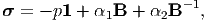
Having established for isotropic materials if Cauchy stress is explicitly related to the deformation gradient, then this relationship would be of the form,
 | (6.64) |
where αi =  i(J1,J2,J3), called the material response functions and
needs to be determined from experiments. Thus, restriction due to
objectivity, has reduced the number of variables in the function from 9 to 3
and the number of unknown functions from 6 to 3. Next, let us see if we
can further reduce the number of variables that the function depends
upon or the number of functions themselves. Since, in an elastic process
there is no dissipation of energy, this reduces the number of unknown
functions to be determined to just one and thus Cauchy stress is given
by13 ,
i(J1,J2,J3), called the material response functions and
needs to be determined from experiments. Thus, restriction due to
objectivity, has reduced the number of variables in the function from 9 to 3
and the number of unknown functions from 6 to 3. Next, let us see if we
can further reduce the number of variables that the function depends
upon or the number of functions themselves. Since, in an elastic process
there is no dissipation of energy, this reduces the number of unknown
functions to be determined to just one and thus Cauchy stress is given
by13 ,
![∂W 2 [∂W ∂W ]
σ = ----1 + --- ----B - ----B -1 ,
∂J3 J3 ∂J1 ∂J2](main751x.png) | (6.65) |
where W = Ŵ(J1,J2,J3), is called as the stored (or strain) energy per unit volume of the reference configuration. Notice that here the stored energy function is the only function that needs to be determined through experimentation.
In practice, the materials undergo a non-dissipative process only when the relative displacements are small, resulting in the components of the displacement gradient being small. Hence, it is of interest to see the implications of this approximation on a general representation for Cauchy stress (6.64).
In chapter 3 (section (3.5.1), we saw that the deformation gradient is related to the Lagrangian and Eulerian displacement gradient as:
 | (6.66) |
Hence, the left Cauchy-Green deformation tensor is given by
 | (6.67) |
If tr(HHt) << 1 and tr(hht) << 1, then we could approximately calculate the left Cauchy-Green deformation tensor as
 | (6.68) |
We also saw in chapter 3 (section 3.8) that when tr(HHt) << 1 and tr(hht) << 1, H ≈ h. Therefore we need not distinguish between the Lagrangian and Eulerian linearized strain. By virtue of these approximations the expressions in equation (6.68) can be written as:
 | (6.69) |
where ϵ denotes the (Lagrangian or Eulerian) linearized strain tensor. Consequently, the invariants are calculated approximately as14
 | (6.70) |
Substituting (6.69) in a general representation for stress in a isotropic material, (6.64) we obtain
 | (6.71) |
where
 | (6.72) |
are functions of tr(ϵ) by virtue of (6.70). It is necessary that α0l should be a linear function of tr(ϵ) and α1l a constant; because we neglected the higher order terms of ϵ to obtain the above expression. Consequently, the expression for Cauchy stress (6.71) simplifies to,
 | (6.73) |
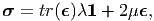
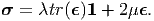
where λ and μ are Lamè constants and these constants alone need to be determined from experiments. The relation (6.73) is called the Hooke’s law for isotropic materials.
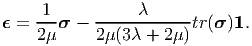
Since, the relation between the Cauchy stress and linearized strain is linear we can invert the constitutive relation (6.73) and write the linearized strain in terms of the stress as,
 | (6.74) |
Taking trace on both sides of equation (6.73) we obtain,
![tr(σ ) = tr(ϵ)[3λ + 2μ ],](main763x.png) | (6.75) |
on noting that tr(⋅) is a linear operator and that tr(1) = 3. Thus, equation (6.74) is obtained by rearranging equation (6.73) and using equation (6.75).
Lamè constants while allows one to write the constitutive relations succinctly, their physical meaning and the methodology for their experimental determination is not obvious. Hence, we define various material parameters, such as Young’s modulus, shear modulus, bulk modulus, Poisson’s ratio, which have a physical meaning and is easy to determine experimentally.
Before proceeding further, a few comments on the Hooke’s law has to be made. From the derivation, it is clear that (6.73) is an approximation to the correct and more general (6.64). Consequently, Hooke’s law does not have some of the characteristics one would expect a robust constitutive relation to possess. The first drawback is that contrary to the observations rigid body rotations induces stresses in the body. To see how this happens, recall from chapter 3 (section 3.10.1) that linearized strain is not zero when the body is subjected to rigid body rotations. Since, strain is not zero, it follows from (6.73) that stress would be present. The second drawback is that the constitutive relation (6.73) does not by itself satisfy the restriction due to objectivity. In fact it is not even Galilean invariant. Given that, due to equivalent placement of the body the displacement gradient transforms as given in equation (6.19) and Cauchy stress transforms as given in equation (6.25), it is evident that the restriction due to non-uniqueness of placers is not met. Despite these drawbacks, it is useful and gives good engineering estimates of the stresses and displacements under applied loads in certain classes of bodies.
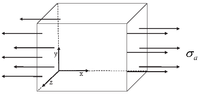
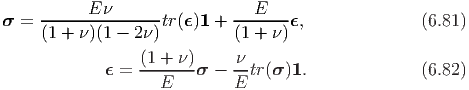
In this section, we define the various material parameters and relate them to the Lamè constants. We do this by defining the stress that is applied on the body in the shape of a cuboid. Since, the body is assumed to obey Hooke’s law, the state of strain gets fixed once the state of stress is specified because of the relation (6.74). Consequently, these parameters can be defined by prescribing the state of strain in the body as well.
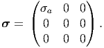
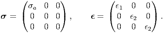
Consider a cuboid being subjected to a uniform normal traction on two of its faces as shown in figure 6.3. Assuming the stress field is uniform, that is spatially constant, the Cartesian components of the stress at any point in the body is,
 | (6.76) |
Substituting the above in equation (6.74) for the stress we obtain the strain as
![( [ ] )
12μ 1 - 3λλ+2μ σa 0 0
ϵ = | ----λ--- |
( 0 - 2μ(3λ+2μ)σa 0 )
0 0 - 2μ(3λλ+2μ)σa](main766x.png) | (6.77) |
Now, Young’s modulus, E, is defined as the ratio of the uniaxial stress to the component of the linearized strain along the direction of the applied uniaxial stress, i.e.,
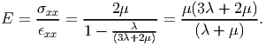 | (6.78) |
The Poisson’s ratio , ν is defined as the negative of the ratio of the component of the strain along a direction perpendicular to the axis of loading, called the transverse strain to the component of the strain along the axis of loading, called the axial strain, i.e.,
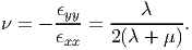 | (6.79) |
In equations (6.78) and (6.79) we expressed the Young’s Modulus and Poisson’s ratio in terms of the Lamè constants. This relation can be inverted to express Lamè constants in terms of E and ν as,
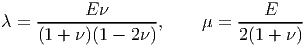 | (6.80) |
Finally, substituting equation (6.80) in equation (6.73) and (6.74), the constitutive relations can be written in terms of the Young’s modulus and Poisson’s ratio as,
Consider a cuboid being subjected to uniform pure shear stress of the form
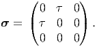 | (6.83) |
Substituting the above state of stress in (6.74), the state of strain is obtained as,
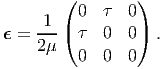 | (6.84) |
In chapter 3, section 3.10.3, we showed that if the angle change between two line segments oriented along X and Y direction is κ, then this simple shearing deformation results in,
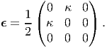 | (6.85) |
Then, the shear modulus, G is defined as the ratio of the shear stress (τ) to change in angle (κ) due to this applied shear stress between two orthogonal line elements in the plane of shear i.e.,
 | (6.86) |
Using equation (6.80b), the shear modulus can be written in terms of the Young’s modulus and Poisson’s ratio as,
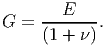 | (6.87) |
Consider a cuboid being subjected to uniform pure hydrostatic stress,
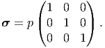 | (6.88) |
Using (6.74) it could be seen that the above state of stress result in the strain tensor being,
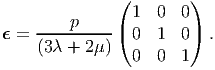 | (6.89) |
The bulk modulus, K, is defined as the ratio of the mean hydrostatic stress to the volumetric strain when the body is subjected to pure hydrostatic stress. Thus,
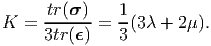 | (6.90) |
Now, we would like to express the bulk modulus in terms of Young’s modulus and Poisson’s ratio. Towards this, we substitute equation (6.80) in (6.90) to obtain
 | (6.91) |
Next, we would like to limit the range of values that these material parameters can take so that the response predicted by using these constitutive relations confirm with the observations.
Let us now see why Young’s and shear modulus cannot be ∞. From the definition of the Young’s modulus we find that the axial displacement due to an applied axial load has to be zero if E = ∞. Similarly, if G = ∞ the change in angle due to an applied shear stress is zero. These would happen only if the body is rigid since, no strain develops despite stress being applied. However, the focus of the study here is deformable bodies. Hence, we obtain the condition that E < ∞, G < ∞.
However, the bulk modulus can be ∞. From the definition of bulk modulus, it is clear that if K = ∞ for some material, then the volumetric strain developed due to applied hydrostatic pressure, for these materials has to be zero. This means that the volume of the body made of this material does not change, the material is incompressible. Some materials like rubber, polymers are known to be nearly incompressible. Moreover, it is also known that the volume of these materials do not change in any deformation. This means that these materials are capable of undergoing only isochoric deformations. Constitutive relations for such incompressible materials are obtained in section 6.7.1.
Since, we expect that tensile stress produce elongation and compressive stresses produce shortening, the three modulus - Young’s, shear and bulk - should be positive. Since, E is positive, for G to be positive and finite, equation (6.87) requires (1 + ν) > 0. Thus,
 | (6.92) |
Note that, this is a strict inequality because if (1 + ν) = 0, G = ∞, (since 0 < E < ∞) which is not permissible.
Similarly, for K to be positive, it transpires from equation (6.91) that (1 - 2ν) ≥ 0, since E is positive. Hence,
 | (6.93) |
Here we allow for equality because K can be ∞.
Combining these both restrictions (6.92) and (6.93) on the Poisson’s ratio,
 | (6.94) |
Thus, Poisson’s ratio can be negative, and it has been measured to be negative for certain foams. What this means is that as the body is stretched along a particular direction, the cross sectional area over which the load is distributed can increase. However, for most materials, especially metals, this cross sectional area decreases and therefore the Poisson’s ratio is positive.
Finally, we show that the three modulus values cannot be zero. From the definition of these modulus, they being zero means that, any amount of strain can develop even when no stress is applied. This means that there can be displacement without the force, when the modulus value is zero. Since, there has to be force for displacement, this means that the modulus cannot be zero.
In table 6.1 the restrictions on various parameters are summarized. The point to note is that one of the Lamè constants, λ has no restrictions. From equation (6.80), it can be seen that if 0 ≤ ν ≤ 0.5, then from the restrictions on E and ν it can be said that λ ≥ 0. However, λ < 0 for certain foams whose Poisson’s ratio is negative. Therefore λ has no restrictions.
| Material Parameter | Symbol | Restriction |
| Young’s modulus | E | 0 < E < ∞ |
| Shear modulus | G | 0 < G < ∞ |
| Bulk modulus | K | 0 < K ≤ ∞ |
| Poisson’s ratio | ν | -1 < ν ≤ 0.5 |
Lamè constant | μ | 0 < μ < ∞ |
| λ | -∞ < λ < ∞ | |
Till now we have been focusing on materials that have no internal constraint, that is, if the required body force and boundary traction can be applied, any smooth displacement field can be realized in bodies made of these materials. However, in some materials this is not true. Only smooth displacement fields that satisfy certain constraints are realizable. The most common constraint on the displacement field is that it be volume preserving. Contrary to the reality, beginners tend to think that in all materials volume is preserved in all feasible deformations just because the cross sectional area reduces when uniaxially stretched. However, this is not true. We show this next. Recollecting from chapter 3 (section 3.6) that the ratio of the deformed volume, v to the original volume, V in case of homogeneous deformation is given by,
 | (6.95) |
where we have used equation (6.70c) to approximately compute det(F) when the components of the displacement gradient are small. Using equation (6.77) that gives the state of strain in the cuboid subjected to uniaxial stress, σa, the change in its volume is computed to be
 | (6.96) |
where the last two equalities are obtained using equation (6.90) and (6.91). Thus, it is apparent that the volume of the cuboid changes as the magnitude of the uniaxial stress changes when ν ≠ 0.5. For physically possible values of Poisson’s ratio, other than 0.5, the volume increases when uniaxially stretched and decreases when compressed.
In this section, we outline general principle to generate constitutive relations for internally constrained materials. Assuming that the materials internal constraint can be given by a equation of the form,
 | (6.97) |
where is a scalar valued function. The requirement that the internal constraint (6.97) be objective necessitates
 | (6.98) |
For (6.98) to hold:
 | (6.99) |
where Ji are the invariants of B as defined in (6.33). The proof for this is left as an exercise; the steps leading to this is similar to that used to obtain the constitutive representation for Cauchy stress.
In order to accommodate its motion to an internal constraint a material body must be able to bring appropriate contact forces into play and the constitutive equation governing its stress response must be such as to allow these forces to act. Thus, the stress at a point x and time t is uniquely determined by the value of the deformation gradient to within a symmetric tensor A which is not determined by the motion of the body and which does no work in any motion compatible with the constraints, i.e.,
 | (6.100) |
where αi =  i(J1,J2,J3) are the same material response functions as defined
before in (6.32) and Ji’s are invariants of B defined in (6.33).
i(J1,J2,J3) are the same material response functions as defined
before in (6.32) and Ji’s are invariants of B defined in (6.33).
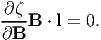
It can be shown that15 , the rate at which the applied stresses does work is given by the expression σ ⋅ l, where l = grad(v), the Eulerian gradient of the velocity field. Hence, the requirement that A do no work requires that
 | (6.101) |
for all allowable motions. To relate A with  we take material time derivative of
(6.99) to obtain
we take material time derivative of
(6.99) to obtain
 | (6.102) |
Now let
 | (6.103) |
where p is an arbitrary scalar to be determined from boundary conditions and/or equilibrium equations. While it is easy to show that, the above choice for the constraint stress satisfies the requirement (6.101), it is difficult to show that this is the only choice and is beyond the scope of this course.
Hence, a general representation for stress with kinematic constraint (6.99) is given by
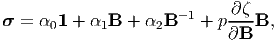 | (6.104) |
with a undetermined scalar p to be found using equilibrium equations and/or boundary conditions.
As already discussed, material that can undergo only isochoric motions is called incompressible material. As was shown in chapter - 3 for isochoric motions, det(F) = J3 = 1. Hence,
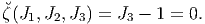 | (6.105) |
Substituting (6.105) in (6.103) and using (2.189) we obtain
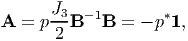 | (6.106) |
where p* = -p∕2. Consequently, a general representation for Cauchy stress (6.104) for incompressibility constraint reduces to,
 | (6.107) |
where now, αi = αi(J1,J2) since J3 is identically 1. Now introducing, p+ = -α 0 + p*, we obtain
 | (6.108) |
where without any loss of generality we assume p+ to be some arbitrary scalar to be determined from boundary conditions and/or equilibrium equations. For convenience and brevity in notation we shall drop the superscript + in p+ and write
 | (6.109) |
which we consider as the most general representation for Cauchy stress in an incompressible material being subjected to elastic deformation.
As before (see section 6.4), it can be shown that when the components of the displacement gradient is small, the kinematical constraint equation (6.105) reduces to requiring,
 | (6.110) |
and consequently the equation (6.109) can be approximated as,
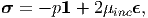 | (6.111) |
where μinc is a constant material parameter and p is an arbitrary scalar to be determined from equilibrium equations and/or boundary condition. Equation (6.111) is the constitutive relation for an incompressible material undergoing elastic deformation such that the components of the displacement gradient are small.
Before concluding this section, we would like to find the value of all the material parameters defined in section 6.5 for this incompressible material.
In case of the cuboid being subjected to uniaxial stress, the state of stress and strain are:
 | (6.112) |
The incompressibility condition (6.110) requires that
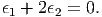 | (6.113) |
Hence, the incompressible materials Poisson’s ratio,
 | (6.114) |
Substituting (6.112) along with the requirement that ϵ2 = -ϵ1∕2 obtained from (6.113) for stress and strain in (6.111) we obtain:
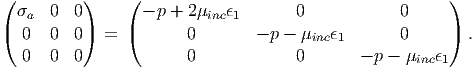 | (6.115) |
For the above equation to hold, p = -μincϵ1 and hence, σa = 3μincϵ1. Thus, the incompressible materials Young’s modulus,
 | (6.116) |
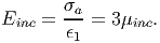
If the cuboid is being subjected to pure shear state of stress and strain,
 | (6.117) |
then it is straightforward to verify that for this state of strain tr(ϵ) = 0 and therefore the incompressibility condition (6.110) is met. Substituting, (6.117) in (6.111) we obtain:
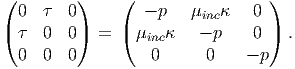 | (6.118) |
For this equation to hold, p = 0 and τ = μincκ. Now, the incompressible shear modulus is,
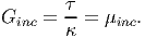 | (6.119) |
Finally, if a incompressible cuboid is subjected to hydrostatic pressure, σ = -p1 and ϵ = 0, for the incompressibility constraint (6.110) and the constitutive relation (6.111) to hold. Thus, incompressible materials bulk modulus, Kinc = ∞.
Understandably there is only one material parameter in (6.111). The incompressibility constraint (6.110) requires that νinc = 0.5 or equivalently, Kinc = ∞ there by fixing one of the two independent material parameters in the isotropic Hooke’s law.
As you would have noticed, for incompressible materials, both the state of stress and strain are prescribed and found necessary to solve certain boundary value problems. On the other hand for unconstrained materials only stress (or strain) needs to be specified for the same boundary value problems. Hence, the solution techniques used for solving unconstrained materials is different from that of constrained materials. In the remainder of this course we focus on the unconstrained materials.
From the above exposition it would have been clear that isotropic Hooke’s law is an approximation to a more general theory. We could proceed in a similar fashion to obtain orthotropic Hooke’s law. On the other hand, as is done in many textbooks on linearized elasticity, we can begin by stating that the Cauchy stress is linearly related to the linearized strain, impose the restriction due to material symmetry on this constitutive relation and obtain isotropic or orthotropic Hooke’s law. However, there are some differences in the orthotropic Hooke’s law obtained by these two approaches. Without develing into these differences, in this section we obtain the orthotropic Hooke’s law by the second approach.
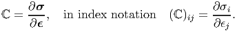
Since, we assume that the second order tensor stress is linearly related to another second order tensor, the strain, we say that the stress is obtained by the action of a fourth order tensor on strain,
 | (6.120) |
where ℂ is the fourth order elasticity tensor. Equivalently, one may invert the equation (6.120) to write strain in terms of stress as,
 | (6.121) |
where D is the fourth order elastic compliance tensor.
Recalling from chapter 2 (section 2.4) the fourth order tensor has 81 components. As discussed in section 2.4.1, for the following discussion it is easy to view second order tensors as column vectors with 9 components and fourth order tensors as 9 by 9 matrix. By virtue of the stress and strain being symmetric tensors, with only six independent components equation (6.120) can be written as,
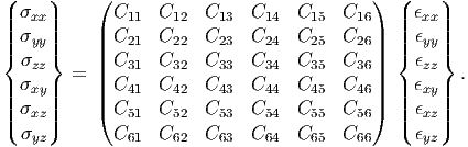 | (6.122) |
Thus, of the 81 components only 36 are independent.
As stated before, since elastic process is non-dissipative, the stress is derivable from a potential called the stored (or strain) energy, W as,
 | (6.123) |
where W = Ŵ(ϵ). The above equation in index notation is given by
 | (6.124) |
when the stress and strain tensors are represented as column vectors with six components. Now, σ1 = σxx, σ2 = σyy, σ3 = σzz, σ4 = σxy, σ5 = σxz, σ6 = σyz and ϵ1 = ϵxx, ϵ2 = ϵyy, ϵ3 = ϵzz, ϵ4 = ϵxy, ϵ5 = ϵxz, ϵ6 = ϵyz. This is just a change in notation.
It follows from (6.120) that the elasticity tensor could be obtained from
 | (6.125) |
Substituting (6.124) in the above equation,
 | (6.126) |
Thus, if W is a smooth function of strain, which it is, then the order of differentiation would not matter. Hence, elasticity tensor would be a symmetric fourth order tensor. This means that the number of independent components in ℂ reduces from 36 to 21 components.
Further reduction in the number of independent components of the elasticity tensor cannot be done by restriction due to non-uniqueness of placers argument. Given that, due to equivalent placement of the body the displacement gradient transforms as given in equation (6.19) and Cauchy stress transforms as given in equation (6.25), it is evident that the restriction due to non-uniqueness of placers is not met by the constitutive relation (6.120). Then, due to changes in the coordinate basis, the elasticity tensor should transforms as
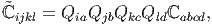 | (6.127) |
according to the transformation law for fourth order tensor (see section 2.6). Ideally we should require that the components of the elasticity tensor be the same irrespective of the choice of the basis. In other words, this means, as discussed in section 2.6.3, that the elasticity tensor should be the isotropic fourth order tensor. Since, the elasticity fourth order tensor is symmetric, in the general representation for the isotropic fourth order tensor (2.165), γ = β = μ and thus,
![¯
ℂ = λ1 ⊗ 1 + μ[I + I],](main818x.png) | (6.128) |
where we have replaced the constant α with λ. This λ and μ are the same Lamè constants. Writing (6.128) in matrix form,
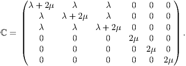 | (6.129) |
Thus, we have obtained the isotropic form of the Hooke’s law.
Contrary to this ideal requirement, it is required that the components of
the elasticity tensor be the same only for certain equivalent choices of
the basis vectors. A material with three mutually perpendicular planes
of symmetry is called orthotropic. This means that 180 degree rotation
about each of the coordinate basis should not change the components of
the elasticity tensor. Thus, for an orthotropic material the components
of  must be same as that of ℂ in (6.127) for the following choices of
Qpq:
must be same as that of ℂ in (6.127) for the following choices of
Qpq:
![( ) ( ) ( )
- 1 0 0 1 0 0 - 1 0 0
[Q ]pq = ( 0 - 1 0) , [Q ]pq = ( 0 - 1 0 ) , [Q ]pq = ( 0 1 0 ) .
0 0 1 0 0 - 1 0 0 - 1](main821x.png) | (6.130) |
It can be seen that as a result of this condition, the number of independent components in the elasticity tensor reduces from 21 to 9 for an orthotropic material and hence ℂ for an orthotropic material is given by:
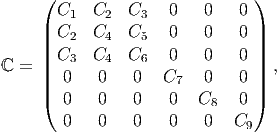 | (6.131) |
where C1, C2, …, C9 are material parameters.
Similarly, for other equivalent choices of the basis vector, we obtain different forms for the elasticity tensor.
One can now define material parameters like Young’s modulus, Poisson’s ratio, shear modulus and elaborate on the experiments that needs to be done to estimate the 9 constants characterizing the orthotropic material. Then, one can look at restrictions on them. Instead of doing these, we now focus on solving boundary value problems involving isotropic materials that obey Hooke’s law.
In this chapter, we saw what a constitutive relation is? why do we need constitutive relations? Then we understood what we mean by an elastic response. This was followed by a discussion on the general restrictions that the constitutive relation has to satisfy and its application to get a general representation for Cauchy stress in an isotropic material undergoing elastic process. When the components of the displacement gradient are small, we showed that this general representation reduces to isotropic Hooke’s law. Then, we introduced the various material parameters used to express the Hooke’s law and established the relationship between them. We also found physically reasonable range of values that these parameters can take. While all these were dealt with in detail, we looked briefly on how to obtain constitutive relations for materials with constraints. As an illustration of this methodology, we obtained the constitutive relation for incompressible materials, materials which undergo only isochoric deformations. Finally, we also derived the Hooke’s law for orthotropic materials. The one equation that should be remembered from this chapter is:
 | (6.132) |
= {(X,Y,Z)|0 ≤ X ≤ 1cm, 0 ≤ Y ≤ 1cm, 0 ≤ Z ≤ 1cm}
obeying isotropic Hooke’s law with Young’s modulus, E = 200 GPa
and Poisson’s ratio, ν = 0.3 is subjected to an uniform Cauchy
stress,
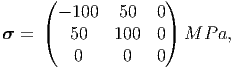 |
corresponding to an orthonormal Cartesian basis ({ex,ey,ez}). For this cube:
 = {(X,Y,Z)|0 ≤ X ≤ 1cm, 0 ≤ Y ≤ 1cm, 0 ≤ Z ≤ 1cm}
obeying isotropic Hooke’s law with Young’s modulus, E = 200 GPa
and Poisson’s ratio, ν = 0.3 is subjected to an uniform Cauchy
stress,
= {(X,Y,Z)|0 ≤ X ≤ 1cm, 0 ≤ Y ≤ 1cm, 0 ≤ Z ≤ 1cm}
obeying isotropic Hooke’s law with Young’s modulus, E = 200 GPa
and Poisson’s ratio, ν = 0.3 is subjected to an uniform Cauchy
stress,
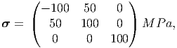 |
corresponding to an orthonormal Cartesian basis ({ex,ey,ez}). For this cube find parts (a) through (m) in problem 5.
 .
.
 x,
x, y,
y, z}. The new basis is obtained by rotating an angle 30
degrees in the clockwise direction about ez axis.
z}. The new basis is obtained by rotating an angle 30
degrees in the clockwise direction about ez axis.
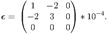 | (6.133) |
For this constant strain field, solve parts (a) through (n) in problem 7.
= {(X,Y,Z)|0 ≤ X ≤ 1, 0 ≤ Y ≤ 1, 0 ≤ Z ≤ 1}
in the reference configuration, is subjected to the following linearized strain
field:
 | (6.134) |
where A, B, C, D are constants. Find conditions, if any, on the constants if this strain field is to be obtained from a smooth displacement field of the cube. For this value of the constants, find the stress field if the cube obeys isotropic Hooke’s law with Young’s modulus, E = 200 GPa and Poisson’s ratio, ν = 0.3 and verify if this stress field satisfies the equilibrium equations assuming that there are no body forces acting on the cube and that the cube is in static equilibrium.