denote the abstract body, that is the set of particles that constitute the
body. Assuming that the body is made of only 8 particles we write
denote the abstract body, that is the set of particles that constitute the
body. Assuming that the body is made of only 8 particles we write
Kinematics is the study of motion, regardless of what is causing it. All bodies in this universe are in motion. Hence, it becomes important to understand how the motion can be described or abstracted mathematically. First, we shall strive to develop an intuitive understanding of certain primitive concepts, namely, body, position and time. Then, we shall proceed to define motion, displacement and velocity fields. Here we shall see that there are two ways of mathematically representing these fields, called the material description and spatial description. Then, we shall dwell on kinematical considerations which are basic to solid mechanics.
Intuitively we understand what a body is. We think that the body is made of a number of particles. Picking up some arbitrary particle we can talk about particles that are on top or below this particle, in front or behind this particle, and to the right or left of this particle. This relationship between the particles is maintained in all motions of the body, that is if two particles is on two different sides of another particle, these two particles stay on either side of the other particle for any motion of the body. Therefore, we say that the body is made up of ordered particles. If the number of particles is countless then the body is described as a continuum and when it is countable it is described to be discrete.
Now, we want to express these intuitive notions of the body in the language of mathematics. The mathematical analogue of the material particle is the point. Mathematically, by point we mean a collection of ‘n’ (real) numbers, for our purposes here. Assuming that we have a scale to measure the distance, then to identify other particles from a given particle, we need to give three distances, namely the distance on top, to the right and in the front of that particular particle. Hence, for each point we have to associate three numbers corresponding to the three distances mentioned above. Therefore the points are said to belong to a three dimensional space, since the value of n is 3. If we use a linear scale, which is the usual practice, to measure the distance then we say that the points belong to a 3D Euclidean space or more specifically 3D Euclidean translation space, also sometimes referred to as 3D Euclidean point space. Further, in the language of mechanics, this mapping of the particles to points in the 3D Euclidean space is called a placer and is denoted by κ.
Though one might understand what a body is intuitively, some choices made here to mathematically represent it needs deliberation. For this we need to understand the mathematical notion of a “point”. Though we associate - ⋅ - it as a point. It is not. ⋅ is at best a collection of points. Point by definition is a limiting sphere obtained when the radius of the sphere tends to zero. Thus one cannot see a point; its volume is also zero. Stacking of points along one direction alone yields a line, stacking of lines along a direction perpendicular to the direction of the line yields a plane, stacking of planes along the normal direction to the plane yields a 3D cube which alone can be seen and has a volume. Thus, one should realize that by stacking countless number of points of zero volume we have created a finite volume, as a consequence of limiting process. Consequently, the same1 countless number of points could occupy different volumes at different instances in time.
It should be clear from the above discussion that particle is not a chunk of material that many believe it to be. This is because the particle is mapped on to the mathematical idea of a point which as we saw above has zero volume.
Let denote the abstract body, that is the set of particles that constitute the
body. Assuming that the body is made of only 8 particles we write
 | (3.1) |
meaning that the eight particles are mapped on to the points (0, 0, 0), (1, 0, 0),
(1, 1, 0), (0, 1, 0), (0, 0, 1), (1, 0, 1), (1, 1, 1), (0, 1, 1). The right hand side of the
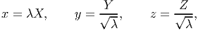
equation (3.1) means the following: Take an element each from the set X, Y and Z
and form a new set called which is the collection of these three elements.
Mathematically, this is stated as: the set is obtained by taking the Cartesian
product2
of the sets X, Y and Z. The elements in the set X are 0 and 1 and that in the set
Y and Z are also 0 and 1. The elements in the set need not be discrete they can be
continuous also. In fact, they have to be continuous when the body is a
continuum.
Thus, for the body made up of countless number of material particles, we write
 | (3.2) |
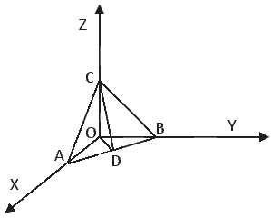
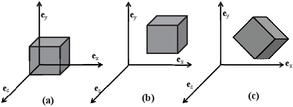
By this, we mean that each point within the unit cube is occupied by a material particle belonging to the body. Since the body occupies contiguous region in space it is apt that it is described as a continuum. Pictorially this configuration of the body is represented as shown in figure 3.1a.
It is just incidental that one of the vertex of the cube coincides with the point (0, 0, 0). Another person can map the same body onto a different region of the Euclidean space and thus he might write
 | (3.3) |
where, X0, Y 0, Z0 are some constants. This representation of the unit cube is shown pictorially in figure 3.1b. In fact, it is not necessary that the cube be oriented such that the normal to its faces coincide with the Cartesian coordinate basis, it can make an angle with the coordinate basis too, as shown in figure 3.1c. This configuration of the body is analytically expressed as:
 | (3.4) |
Before proceeding further, we recap the properties of the placers. First, the placers are one to one functions that is each material particle gets mapped on to a unique point in the 3D Euclidean space. However, there is no unique placer for a given body. Different persons can map a given body to different regions of Euclidean point space. We shall later see how this non-uniqueness of placers is built into the theory developed to describe the mechanical response of the bodies.
While defining bodies in equations (3.1) through (3.4) we tacitly assumed that the point space corresponded to Cartesian coordinates. This specification of the coordinate system is important to arrive at the formula to be used to compute the distance between two triplets. Recognize that if we are using the same formula to obtain the distance between two triplets in different coordinate systems, it is equivalent to using different scales to measure the distance.
Many a times, the choice of coordinate system is made so that we can define the body succinctly. For example, consider a body in the shape of an annular (or solid) right circular cylinder of length, H. Using cylindrical polar coordinates, (R, Θ,Z), this body is mathematically defined as:
 | (3.5) |
where Ri and Ro are some positive constants, with Ri = 0 for a solid cylinder. Try defining this body using Cartesian coordinates.
Experience has shown that it is easier to do computations if we use vector
space instead of point space. Naively, while in vector spaces we speak of position
vectors of a point, in point space we speak about the coordinates of a point. Next,
we would like to establish this relationship between the mathematical
ideas of the vector space and point space. To do this, for each ordered
pair of points (a,b) in the Euclidean point space  there corresponds a
unique vector in the Euclidean vector space, 𝔙, denoted by
there corresponds a
unique vector in the Euclidean vector space, 𝔙, denoted by  , with the
properties
, with the
properties
 = -
= - , ∀ a, b ∈.
 =
=  +
+  , ∀ a, b, c ∈.
, and a Cartesian coordinate basis
to span the vector space, 𝔙, there corresponds to each vector a ∈𝔙 a
unique point a ∈ such that a =
, ∀ a, b, c ∈.
, and a Cartesian coordinate basis
to span the vector space, 𝔙, there corresponds to each vector a ∈𝔙 a
unique point a ∈ such that a =  , the point o is called the origin
and a the position of a relative to o.
, the point o is called the origin
and a the position of a relative to o.In other words, property (iii) states that the components of any vector a (a1,a2,a3)
relative to a chosen Cartesian coordinate basis correspond to the coordinates of
some point a in . The fact that this holds only for Cartesian coordinate system
cannot be overemphasized. To see this, recall that in cylindrical polar coordinate
system even though a triplet (R, Θ,Z) characterizes a point in , position
vectors have components of the form (R, 0,Z) only. That is the components
of the position vector of a point is not same as the coordinates of the
point.
The notions of distance and angle in are derived from the scalar product on
the supporting vector space 𝔙: the distance between the arbitrary points a and b
is defined by | | and the angle, α subtended by a and b at a third arbitrary point
c by
| and the angle, α subtended by a and b at a third arbitrary point
c by
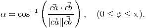 | (3.6) |
Thus, the choice of scale corresponds to the different expressions for the scalar product.
Considering the physical body to be made up of material particles, denoted by
P, we have seen how it can be mapped to the 3D Euclidean point space and hence
to the 3D Euclidean vector space. Thus, the region occupied by this body in the
3D Euclidean vector space is called as the configuration of the body and is
denoted by 𝔅. Then, the placing function κ: →𝔅 and its inverse κ-1: 𝔅 →
are defined as:
 | (3.7) |
Recognize that the inverse exist because the mappings are one to one by definition. Henceforth, by placer we mean placing the body in the Euclidean vector space not the point space.
Next, let us understand what time is. Time concerns with the ordering of events. That is, it tells us whether an event occurred before or after a particular event. We shall assume that we cannot count the number of events. Hence, we map the events to the points on a real line. This assumption that the number of events is countless, is required so that we can take derivatives with respect to time. The part of the real line that is used to map a set of events is the prerogative of the person who establishes this correspondence which is similar to the mapping of the body on to the 3D Euclidean point space. The motion of a body is considered to be an event in mechanics. When a body moves, its configuration changes, that is the region occupied by the body in the 3D Euclidean vector space changes.
Let t be a real variable denoting time such that t ∈ ⊆
⊆ , set of reals. If we
could associate a configuration, 𝔅t for the body for each instant of time in the
interval of interest then the family of configurations {𝔅t : t ∈} is called motion
of . Hence, we can define functions ϕ: × →𝔅t and ϕ-1: 𝔅
t × → such
that
, set of reals. If we
could associate a configuration, 𝔅t for the body for each instant of time in the
interval of interest then the family of configurations {𝔅t : t ∈} is called motion
of . Hence, we can define functions ϕ: × →𝔅t and ϕ-1: 𝔅
t × → such
that
 | (3.8) |
In a motion of a typical particle, P occupies a succession of points which
together form a curve in . This curve is called the path of P and is given in a
parametric manner by equation (3.8a). The velocity and acceleration of P are
defined as rate of change of position and velocity with time, respectively, as P
traverses its path.
While the definition of motion by (3.8a) is satisfactory, it would be useful if it were to be a function of the vectors instead of points. To achieve this we make use of the equation (3.7b). That is we choose a certain configuration of the body and identify the particles by the position vector of the point it occupies in this configuration, then
 | (3.9) |
χκ is called the motion field and the subscript κ denotes that it depends on the configuration which is used to identify the particles. The configuration in which the particles are identified is called the reference configuration and is denoted by 𝔅r. This definition does not require the reference configuration to be a configuration actually occupied by the body during its motion. If the reference configuration were to be a configuration actually occupied by the body during its motion at some time to, then (3.9) could be obtained from (3.8) as
 | (3.10) |
We call χκ (or χto) the deformation field when it is independent of time or its dependence on time is irrelevant.
Now, we would like to make a few remarks. The definition of a body and motion is independent of whether we are concerned with rigid body or deformable body. However, certain structures or details impounded on the body depends on this choice. Till now, we have been talking about the body being a set of particles but to be precise we should have said material particles. This detail is important within the context of deformable bodies, as we shall see later. It should also be remembered that the distinction that a given particle is steel or wood is made right in the beginning. Thus, within the realms of classical mechanics we cannot model chemically reacting body where material particles of a particular type gets transformed into another. Because the body is considered to be a fixed set of material particles, they cannot die or be born or get transformed.
As we shall see later, an important kinematical quantity in the study of
deformable bodies is the gradient of motion. For us to be able to find the gradient
of motion, we require the motion field, (3.9) to be continuous on and there
should exist countless material particles of the same type (material) in spheres of
radius, r for any value of r less than δo where δo is some constant. It is for this
purpose, in the study of deformable bodies we require the body to be a
continuum.
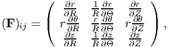
The gradient of motion is generally called the deformation gradient and is denoted by F. Thus
 | (3.11) |
Since, χ is a function of both X and t we have used a partial derivative in the definition of the deformation gradient. Also, we haven’t defined it as Grad(x) because for the Grad operator, as defined in chapter 2, the range of the function for which gradient is sought is any vector; not just position vectors. The difference becomes evident in curvilinear coordinate systems like the cylindrical polar coordinates.
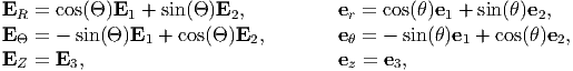
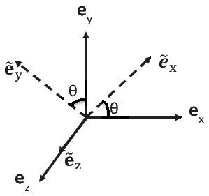
Let {Ei} be the three Cartesian basis vectors in the reference configuration and {ei} the basis vectors in the current configuration. Then, the deformation gradient is written as
 | (3.12) |
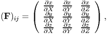
In general, the basis vectors ei and Ej need not be the same. Since the deformation gradient depends on two sets of basis vectors, it is called a two-point tensor. It is pertinent here to point out that the grad operator as defined in chapter 2 (2.207), is not a two-point tensor either. The matrix components of the deformation gradient in Cartesian coordinate system is
 | (3.13) |
where (X,Y,Z) and (x,y,z) are the Cartesian coordinates of a typical material particle, P in the reference and current configuration respectively. Similarly, the matrix components of the deformation gradient in cylindrical polar coordinate system is:
 | (3.14) |
where (R, Θ,Z) and (r,θ,z) are the cylindrical polar coordinates of a typical material particle, P in the reference and current configuration respectively. Substituting
in (3.13) we obtain
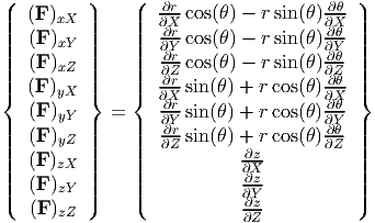 | (3.16) |
where

In the development of the basic principles of continuum mechanics, a body is
endowed with various physical properties which are represented by scalar or
tensor fields, defined either on a reference configuration, 𝔅r or on the current
configuration 𝔅t. In the former case, the independent variables are the position
vectors of the particles in the reference configuration, X and time, t. This
characterization of the field with X and t as independent variables is called
Lagrangian (or material) description. In the latter case, the independent variables
are the position vectors of the particles in the current configuration, x and time, t.
The characterization of the field with x and t as independent variables is called
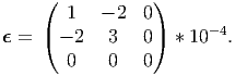
Eulerian (or spatial) description. Thus, density, displacement and stress are
examples of scalar, vector and second order tensor fields respectively and can be
represented as
To understand the difference between the Lagrangian description and Eulerian description, consider the flow of water through a pipe from a large tank. Now, if we seed the tank with micro-spheres and determine the velocity of these spheres as a function of time and their initial position in the tank then we get the Lagrangian description for the velocity. On the other hand, if we choose a point in the pipe and determine the velocity of the particles crossing that point as a function of time then we get the Eulerian description of velocity. While in fluid mechanics we use the Eulerian description, in solid mechanics we use Lagrangian description, mostly.
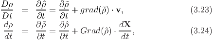
Next, we define what is called as the material time derivative or Lagrangian
time derivative or total time derivative and spatial time derivative or Eulerian
time derivative. It could be inferred from the above that various variables of
interest are functions of time, t and either X or x. Hence, when we differentiate
these variables with respect to time, we can hold either X a constant or x a
constant. If we hold X a constant while differentiating with time, we
call such a derivative total time derivative and denote it by  . On the
other hand if we hold x a constant, we call it spatial time derivative and
denote it by
. On the
other hand if we hold x a constant, we call it spatial time derivative and
denote it by  . Thus, for the scalar field defined by, say (3.20) we have
 . The above equations are obtained by
using the chain rule. Similarly, for a vector field defined by (3.21) we have
. The above equations are obtained by
using the chain rule. Similarly, for a vector field defined by (3.21) we have
 = o and
  = o.
= o.
Finally, a note on the notation. If the starting letter is capitalized for any of the operators introduced in chapter 2 then it means that the derivative is with respect to the material coordinates, i.e. X otherwise, the derivative is with respect to the spatial coordinates, i.e. x. In the above, we have already used this convention for the gradient operator.
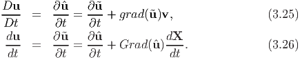
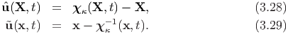
The vector field, u, defined as
 | (3.27) |
represents the displacement field, that is the displacement of the material particles initially at X or currently at x depending on whether Lagrangian or Eulerian description is used. Thus,
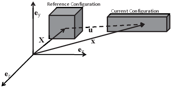
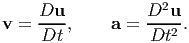
The first and second total time derivatives of the motion field is called the velocity and acceleration respectively. Thus
 | (3.30) |
We note that both the velocity and acceleration can be expressed as a Lagrangian field or Eulerian field. From the definition of the displacement (3.27) it can be seen that the velocity and acceleration can be equivalently written as,
 | (3.31) |
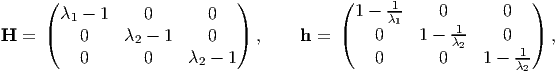
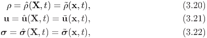
As we have seen before, the displacement field can be expressed as a Lagrangian field or Eulerian field. Thus, we can have a Lagrangian displacement gradient, H and a Eulerian displacement gradient, h defined as
 | (3.32) |
Recognize that these gradients are not the same. To see this, we compute the displacement gradient in terms of the deformation gradient as
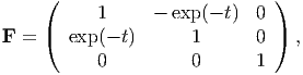
A certain motion of a continuum body in the material description is given in the form:
 | (3.35) |
for t > 0. Find the displacement, velocity and acceleration components in terms of the material and spatial coordinates and time. Also find the deformation and displacement. Assume that the same Cartesian coordinate basis and origin is used to describe the body both in the current and the reference configuration.
It follows from (3.27) that
 | (3.36) |
Similarly, from (3.30) we obtain
Inverting the motion field (3.35) we obtain
![[x + exp (- t)x ] [x - exp (- t)x ]
X1 = --1-----------2-, X2 = --2-----------1-, X3 = x3.
[1 + exp (- 2t)] [1 + exp (- 2t)]](main360x.png) | (3.39) |
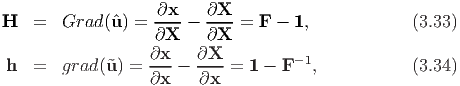
Substituting (3.39) in (3.36), (3.37) and (3.38) we obtain the Eulerian form of the displacement, velocity and acceleration fields as
![[x2 - exp(- t)x1] [x1 + exp(- t)x2]
u˜ = - -----------------exp (- t)E1 + ----------------exp (- t)E2,
[1 + exp(- 2t)] [1 + exp(- 2t)]
[x2---exp-(- t)x1] [x1-+-exp-(- t)x2]
v˜ = [1 + exp (- 2t)] exp (- t)E1 - [1 + exp (- 2t)] exp (- t)E2,
˜a = - [x2---exp(--t)x1]exp (- t)E1 + [x1-+-exp(--t)x2]exp (- t)E2.
[1 + exp(- 2t)] [1 + exp(- 2t)]](main361x.png)
Next, we compute the deformation gradient to be
 | (3.40) |
and the Lagrangian and Eulerian displacement gradient as
![( )
0 - exp(- t) 0
H = ( exp(- t) 0 0 ) , (3.41)
( 0 0 0 )
--exp(-2t)-- - --exp(-t)--- 0
| [1+eexxpp((--t2)t)] [1e+xepx(-p(-2t)2t)] |
h = ( [1+exp(-2t)] [1+exp(--2t)] 0 ) , (3.42)
0 0 0](main363x.png)
Before rigorously deriving the general expressions for transformation of curves, surfaces and volumes, let us obtain these expressions after various simplifying assumptions.
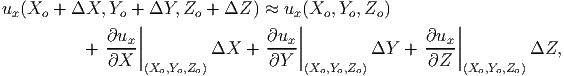
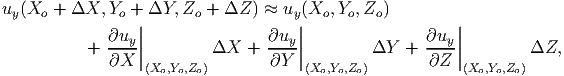
Let us assume the following:
 | (3.43) |
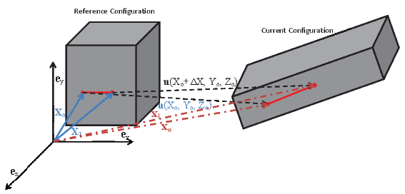
where ux(X,Y,Z), uy(X,Y,Z) and uz(X,Y,Z) are some known functions of the X, Y and Z the coordinates of the material particles in the reference configuration.
 |
 |
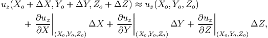 | (3.44) |
First, we are interested in finding how the length of the straight line of length ΔX oriented along the ex direction in the reference configuration of the body, as shown in the figure 3.3 has changed. With the above assumptions, the deformed length of the straight line of length ΔX oriented along the ex direction in the reference configuration is given by,
![∥x1 - xo∥ = ∥X1 - Xo + u(X1 ) - u(Xo )∥
∘ [--------]2---[----]2---[----]2-
= ΔX 1 + ∂ux- + ∂uy- + ∂uz- ,
∂X ∂X ∂X](main369x.png) | (3.45) |
![[ ]
∂ux
∥x1 - xo∥ = ΔX 1 + ∂X-- .](main370x.png) | (3.46) |
Hence, the stretch ratio defined as the ratio of the current length to the undeformed length for a line element oriented along the ex direction is,
![∥x - x ∥
Λ(ex) = ---1----o--
∥X1 - Xo ∥ ∘ --------------------------------
[ ]2 [ ]2 [ ]2 [ ]
= 1 + ∂ux- + ∂uy- + ∂uz- ≈ 1 + ∂ux- .
∂X ∂X ∂X ∂X](main371x.png) | (3.47) |
![[ ∂u ]
Λ (ex) ≈ 1 + --x- .
∂X](main372x.png) | (3.48) |
when the components of the displacement gradient are small. Following a similar procedure, one can determine how the length of line elements oriented along any direction changes. We shall derive a general expression for the same later in section 3.6.1.
Next we are interested in finding how the area of a face of a small cuboid changes due to deformation. Let us assume that the face of the cuboid whose normal coincides with the ez basis is of interest and the sides of this face of the cuboid are of length ΔX along the ex direction and ΔY along the ey direction. Thus, as shown in figure 3.4, Xo (= Xoex + Y oey + Zoez), X1 (= (Xo + ΔX)ex + Y oey + Zoez) and X2 (= Xoex + (Y o + ΔY )ey + Zoez) denote the position vector of the three corners of the face of the cuboid whose normal is ez in the reference configuration and xo, x1 and x2 denote the position of the same three corners of the face of the cuboid in the current configuration. For the same three assumptions listed above, the deformed area of this face of the cuboid is given by,
![a = ∥(x - x ) ∧ (x - x )∥
1 o 2 o
= ∥(X1 - Xo + u(X1 ) - u (Xo )) ∧ (X2 - Xo + u(X2 ) - u(Xo ))∥
||{ [∂uy ∂uz ∂uz ( ∂uy) ]
= (ΔX )(ΔY )|| --------- ---- 1 + ---- ex
[ ∂X ∂(Y ∂X) ] ∂Y
∂uz-∂ux- ∂ux- ∂uz-
+ ∂X ∂Y - 1 + ∂X ∂Y ey
[( ) ( ) ] } |
+ 1 + ∂ux- 1 + ∂uy- - ∂uy-∂ux- e ||,
∂X ∂Y ∂X ∂Y z |](main374x.png) | (3.49) |
 | (3.50) |
Finally, we find the volume of the deformed cuboid. Again recollecting from chapter 2, the box product of three vectors yields the volume of the parallelepiped spanned by them, the deformed volume of the cuboid is given by,
![v = [x1 - xo,x2 - xo,x3 - xo]
{ [( ∂uz ) ( ∂uy ) ∂uy ∂uz ]( ∂ux )
= (ΔX )(ΔY )(ΔZ ) 1 + ---- 1 + ---- - -------- 1 + ----
[ ∂Z ( ∂)Y ] ∂Z ∂Y ∂X
∂uz-∂ux- ∂uz- ∂ux- ∂uy-
+ ∂Y ∂Z - 1 + ∂Z ∂Y ∂X
[ ( ) ] }
+ ∂ux-∂uy- - 1 + ∂uy- ∂ux- ∂uz- ,
∂Y ∂Z ∂Y ∂Z ∂X](main376x.png) | (3.51) |
When the magnitude of the components of the displacement gradient are small, then the deformed volume of the cuboid could be computed from equation (3.51) as,
![[ ∂ux ∂uy ∂uz]
v ≈ (ΔX )(ΔY )(ΔZ ) 1 + ---- + ----+ ---- ,
∂X ∂Y ∂Z](main377x.png) | (3.52) |
by neglecting the quadratic and cubic terms in equation (3.51).
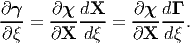
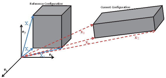
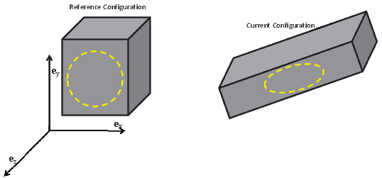
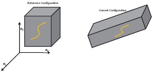
We know the position vector of any particle belonging to the body at various instances of time, t. But now we are interested in finding how a set of contiguous points forming a curve changes its shape. That is, we are interested in finding how a circle inscribed in the reference configuration changes its shape, say into an ellipse, in the current configuration. As we have required the deformation field to be one to one, closed curves like circle, ellipse, will remain as closed curves and open curves like straight line, parabola remains open. The position vectors of the particles that occupy a curve can be described using a single variable, say ξ. For example, a circle of radius R in the plane whose normal coincides with ez, as shown in figure 3.5a would be described as (R cos(ξ),R sin(ξ),Zo), where R and Zo are constants and 0 ≤ ξ ≤ 2π.
Consider a material curve (or a curve in the reference configuration), X = Γ(ξ) ⊂𝔅r, where ξ denotes a parametrization. The material curve by virtue of it being defined in the reference configuration is not a function of time. During a certain motion, the material curve deforms into another curve called the spatial curve, x = γ(ξ,t) ⊂𝔅t, (see figure 3.5b). The spatial curve at a fixed time t is then defined by the parametric equation
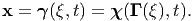 | (3.53) |
We denote the tangent vector to the material curve as ΔX and the tangent vector to the spatial curve as Δx and are defined by
 | (3.54) |
By using (3.53) and the chain rule we find that
 | (3.55) |
Hence, from equation (3.54) and the definition of the deformation gradient, (3.11) we find that
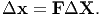 | (3.56) |
Expression (3.56) clearly defines a linear transformation which generates a vector Δx by the action of the second-order tensor F on the vector ΔX. In summary: material tangent vectors map into spatial tangent vectors via the deformation gradient. This is the physical significance of the deformation gradient.
In the literature, the tangent vectors Δx and ΔX, in the current and reference configuration are often referred to as the spatial line element and the material line element, respectively. This is correct only when the curve in the reference and current configuration is a straight line.
Next, we introduce the concept of stretch ratio which is defined as the ratio between the current length to its original length. When we say original length, we mean undeformed length, that is the length of the fiber when it is not subjected to any force. It should be pointed out at the outset that many a times the undeformed length would not be available and in these cases it is approximated as the length in the reference configuration.
In general, the stretch ratio depends on the location and orientation of the material fiber for which it is computed. Thus, we can fix the orientation of the material fiber in the reference configuration or in the current configuration. Corresponding to the configuration in which the orientation of the fiber is fixed we have two stretch measures. Recognize that we can fix the orientation of the fibers in only one configuration because its orientation in others is determined by the motion.
First, we consider deformations in which any straight line segments in the reference configuration gets mapped on to a straight line segment in the current configuration. Such a deformation field which maps straight line segments in the reference configuration to straight line segments in the current configuration is called homogeneous deformation. We shall in section 3.10, illustrate that when the deformation is homogeneous, the Cartesian components of the deformation gradient would be a constant. As a consequence of assuming the curve to be a straight line, the tangent and secant to the curve is the same. Hence, saying that we are considering a material fiber3 of length ΔL initially oriented along A, (where A is a unit vector) and located at P, is same as saying that we are studying the influence of the deformation on the tangent vector, ΔLA at P. Due to some motion of the body, the material particle that occupied the point P will occupy the point p ∈𝔅t and the tangent vector ΔLA is going to be mapped on to a tangent vector with length, say Δl and orientation a. From (3.56) we have
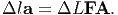 | (3.57) |
Dotting the above equation with Δla, we get
 | (3.58) |
where we have used the fact that a is a unit vector, the relation (3.57) and the definition of transpose. Defining the right Cauchy-Green deformation tensor, C as
 | (3.59) |
and using equation (3.58) we obtain
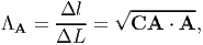 | (3.60) |
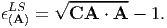
where ΛA represents the stretch ratio of a line segment initially oriented along A. The stretch ratio, ΛA is the one that could be directly determined in an experiment. However, there is no reason why we should restrict our studies to line segments which are initially oriented along a given direction. We can also study about material fibers that are finally oriented along a given direction. Towards this, we invert equation (3.57) to get
 | (3.61) |
Dotting the above equation with ΔLA, we get
 | (3.62) |
using arguments similar to that used to get (3.58) from (3.57). Defining the left Cauchy-Green deformation tensor or the Finger deformation tensor, B as
 | (3.63) |
and using equation (3.62) we obtain
 | (3.64) |
where Λa represents the stretch ratio of a fiber finally oriented along a.
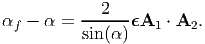
Next, we would like to compute the final angle between two two straight line segments initially oriented along A1 and A2. Recognizing that the angle between two straight line segments, α is computed using the expression:
 | (3.65) |
Using (3.65) and similar arguments as that used to obtain the stretch ratio, it can be shown that the final angle, αf between the straight line segments initially oriented along A1 and A2 is given by
 | (3.66) |
Just, as in the case of stretch ratio, we can also study the initial angle, αi between straight line segments that are finally oriented along a1 and a2. For this case, following the same steps outlined above we compute
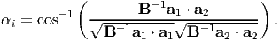 | (3.67) |
We like to record that as in the case of stretch ratio, αi and αf depends on the orientation of the line segments.
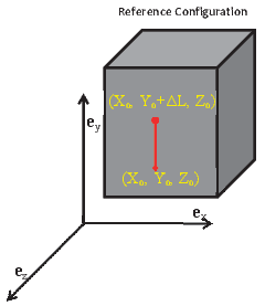 (a) Straight line oriented along Ey at
(Xo,Y o,Zo).
(a) Straight line oriented along Ey at
(Xo,Y o,Zo). 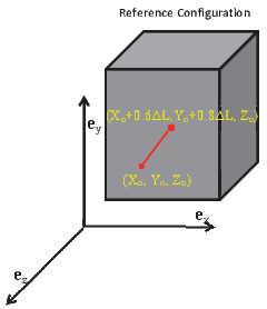 (b) Straight line oriented along (3Ex +
4Ey)∕5 at (Xo,Y o,Zo).
(b) Straight line oriented along (3Ex +
4Ey)∕5 at (Xo,Y o,Zo).
Next, let us see what happens when the deformation is inhomogeneous. For inhomogeneous deformation, the Cartesian components of the deformation gradient would vary spatially and the straight line segment in the reference configuration would have become a curve in the current configuration. Hence, distinction between the tangent and the secant has to be made. Now, the deformed length of the curve, Δl corresponding to that of a straight line of length ΔL oriented along A is obtained from equation (3.56) as,
![∫ ∘ (----)----(----)----(---)--
1 dx- 2 dy- 2 dz- 2
Δl = dξ + dξ + dξ dξ
0 ┌ ----------------------------------------
∫ 1││ [( )2 ( )2 ( )2 ]
= ∘ CA ⋅ A dX-- + dY-- + dZ- dξ,
0 d ξ dξ d ξ](main397x.png) | (3.68) |
 (X(ξ),Y (ξ),Z(ξ)), (X(ξ),Y (ξ),Z(ξ))
denotes the coordinates of the material points that constitutes the straight line
and ξ varies between 0 and 1 to parameterize the straight line. Thus, for a
line oriented along say Ey direction of length ΔL, starting from a point
(Xo,Y o,Zo), (see figure 3.6a) X(ξ) = Xo, Y (ξ) = Y o + ξ(ΔL), Z(ξ) = Zo.
For a line oriented along say (3Ex + 4EY )∕5 of length ΔL, starting from
(Xo,Y o,Zo), (see figure 3.6b) X(ξ) = Xo + 3ξ(ΔL)∕5, Y (ξ) = Y o + 4ξ(ΔL)∕5,
Z(ξ) = Zo. In fact, if one relaxes the assumption that A is a constant
in equation (3.68) then the straight line in the reference configuration
could be a curve and the deformed length could still be calculated from
(3.68).
(X(ξ),Y (ξ),Z(ξ)), (X(ξ),Y (ξ),Z(ξ))
denotes the coordinates of the material points that constitutes the straight line
and ξ varies between 0 and 1 to parameterize the straight line. Thus, for a
line oriented along say Ey direction of length ΔL, starting from a point
(Xo,Y o,Zo), (see figure 3.6a) X(ξ) = Xo, Y (ξ) = Y o + ξ(ΔL), Z(ξ) = Zo.
For a line oriented along say (3Ex + 4EY )∕5 of length ΔL, starting from
(Xo,Y o,Zo), (see figure 3.6b) X(ξ) = Xo + 3ξ(ΔL)∕5, Y (ξ) = Y o + 4ξ(ΔL)∕5,
Z(ξ) = Zo. In fact, if one relaxes the assumption that A is a constant
in equation (3.68) then the straight line in the reference configuration
could be a curve and the deformed length could still be calculated from
(3.68).
Hence, the stretch ratio for the case of inhomogeneous deformation is,
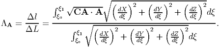 | (3.69) |
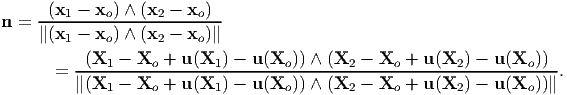
Having seen how points, curves, tangent vectors in the reference configuration gets mapped to points, curves and tangent vectors in the current configuration, we are now in a position to look at how surfaces get mapped. Of interest, is how a unit vector, N normal to an infinitesimal material surface element ΔA map on to a unit vector n normal to the associated infinitesimal spatial surface element Δa.
Let Sr denote the material surface in 𝔅r that is of interest. Then, an element of area ΔA at a point P on Sr is defined through the vectors ΔX and ΔY, each tangent to Sr at P, as ΔAN = ΔX ∧ ΔY where N is a unit vector normal to Sr at P. Due to some motion of the body, the material surface Sr gets mapped on to another material surface St in 𝔅t, the material particle that occupied the point P on Sr gets mapped onto a point p on St and the tangent vectors ΔX and ΔY gets mapped on to another pair of tangent vectors at p denoted by Δx and Δy. Thus, we have
 | (3.70) |
Since, ΔX and ΔY are tangent vectors we have Δx = FΔX and Δy = FΔY. Therefore,
 | (3.71) |
where we have made use of (2.88) and (2.90). Thus, the relation
 | (3.72) |
called Nanson’s formula is an often used expression in continuum mechanics.
Next, we are interested in computing the deformed area, a. For this case, from Nanson’s formula we obtain,
 | (3.73) |
which simplifies to
 | (3.74) |
on using the equation (3.59) and the fact that n is a unit vector. Notice that, once again the deformed area is determined by the right Cauchy-Green deformation tensor.
Next, we seek to obtain the relation between elemental volumes in the reference and current configuration. An element of volume ΔV at a interior point P in reference configuration is given by the scalar triple product [ΔX, ΔY, ΔZ] where ΔX, ΔY and ΔZ are vectors oriented along the sides of an infinitesimal parallelepiped. Since, the point under consideration is interior, we can always find three material curves such that they pass through the point P and ΔX, ΔY and ΔZ are its tangent vectors at P. Now say due to some motion of the body, the material particle that occupied the point P, now occupies the point p, then the curves under investigation would pass through p and the tangent vectors of these curves at this point p would now be Δx, Δy, Δz. Hence,
![Δv = [Δx, Δy, Δz ] = [F ΔX, FΔY, F ΔZ ] = det(F)[ΔX, ΔY, ΔZ ]
= det (F )ΔV,](main405x.png) | (3.75) |
Since det(F) > 0, using the polar decomposition theorem (2.116) the deformation gradient can be represented as:
 | (3.76) |
where R is a proper orthogonal tensor, U and V are the right and left stretch tensors respectively. (These stretch tensors are called right and left because they are on the right and left of the orthogonal tensor, R.) These stretch tensors are unique, positive definite and symmetric.
Substituting (3.76) in (3.59) and (3.63) we obtain
 | (3.77) |
Next, we record certain properties of the right and left Cauchy-Green deformation tensors.
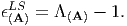
 | (3.78) |
then
 | (3.79) |
Now let na = RNa. Then
 | (3.80) |
Thus, we have shown that εa2 is the principal value for both C and B tensors and Na and RNa are their principal directions respectively.
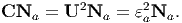
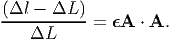
Now, we shall look at the concept of strain. This is some quantity defined by us and hence there are various definitions of the same. Also, as we shall see later, we can develop the constitutive relation independent of these definitions. Experimental observations show that relative displacement of particles alone gives raise to stress. A measure of this relative displacement is the stretch ratio. However, this measure has the drawback that when the body is not deformed the stretch ratio is 1 (by virtue of the deformed length being same as the original length) and hence thought to be inconvenient to formulate constitutive relations. Consequently, another measure of relative displacement is sought which would be 0 when the body is not deformed and less than zero when compressed and greater than zero when stretched. This measure is called as the strain, ϵ(A). There is no unique way of obtaining the strain from the stretch ratio. The following functions satisfy the requirement of the strain:
 | (3.81) |
where m is some real number and ln stands for natural logarithm. Thus, if m = 1 in (1.5a) then the resulting strain is called as the engineering strain, if m = -1, it is called as the true strain, if m = 2 it is Cauchy-Green strain. The second function wherein ϵ(A) = ln(λ(A)), is called as the Hencky strain or the logarithmic strain.
Let us start by looking at the case when m = 2 in equation (3.81), that is the case,
 | (3.82) |
Substituting (3.60) in (3.82) we obtain
 | (3.83) |
where, E = 0.5[C - 1], is called the Cauchy-Green strain tensor. Thus, Cauchy-Green strain tensor carries information about the strain in the material fibers initially oriented along a given direction. Substituting Lagrangian displacement gradient, defined in (3.33), for deformation gradient in the expression for E, we obtain
![1
E = --[H + Ht + HtH ].
2](main414x.png) | (3.84) |
If tr(HHt) << 1, i.e., each of the components of H is close to zero4 , then we can compute E approximately as
![1
E ≈ -[H + Ht ] = ϵL.
2](main415x.png) | (3.85) |
ϵL is called as the Lagrangian linearized strain and will be used extensively while studying linearized elasticity.
Next, we examine the case when m = 1, in equation (3.81), that is the case,
 | (3.86) |
Substituting (3.60) in (3.86) we obtain
 | (3.87) |
Substituting Lagrangian displacement gradient, defined in (3.33), for deformation gradient in the expression for C and using the definition (3.85) for Lagrangian linearized strain, equation (3.87) evaluates to
 | (3.88) |
which when the components of the Lagrangian displacement gradient are small could be approximately computed as
 | (3.89) |
where we have approximately evaluated the square root using Taylor’s series5 . Thus, Lagrangian linearized strain carries the information on changes in length of material fibers initially oriented along a given direction when the changes in length are small.
Instead of studying the strain in fibers oriented initially along a given direction, one can also study strains in fibers finally oriented along a given direction, a. Now, again the following functions satisfy the requirement of the strain:
 | (3.90) |
where m is some real number and ln stands for natural logarithm. We study the case when m = -2 in equation (3.90), that is the case,
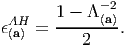 | (3.91) |
Substituting (3.64) in (3.91) and rearranging we obtain
 | (3.92) |
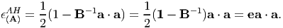
where, e = 0.5[1 - B-1], is called the Almansi-Hamel strain tensor and carries information about the strain in the material fibers finally oriented along a given direction. Substituting Eulerian displacement gradient, defined in (3.34), for F-1 in the expression for e, we obtain
![1 t t
e = 2-[h + h - h h ].](main424x.png) | (3.93) |
If tr(hht) << 1, then we can compute e approximately as
![1- t
e ≈ 2[h + h ] = ϵE.](main425x.png) | (3.94) |
ϵE is called as the Eulerian linearized strain.
The Lagrangian and Eulerian displacement gradients are related through the equation
 | (3.95) |
obtained from the requirement that FF-1 = 1 and substituting the expressions (3.33) and (3.34) for F and F-1 respectively. It immediately transpires that when each of the components of H and h are close to zero then H ≈ h and hence both the Lagrangian and Eulerian linearized strain are numerically the same. Hence, when the distinction is not important the subscript, L or E would be dropped and the linearized strain denoted as ϵ
There are other strain measures called the Hencky strain tensor in the Lagrangian and Eulerian form defined as ln(U) and ln(V) respectively. This strain tensor corresponds the case where the strain along a given direction is defined as the natural logarithm of the corresponding stretch ratio. Hencky strain is also sometimes called as the logarithmic strain.
From now on we shall in this course, study the response of bodies only for cases when the value of the components of both the Lagrangian and Eulerian displacement gradient are small. As we have shown above, this means that not only does the changes in length be small but the rotations also needs to be small. Under these severe but practically reasonable assumptions, the strain-displacement relation is
![[ ]
ϵ = 1-h + ht ,
2](main427x.png) | (3.96) |
where we stop distinguishing between Lagrangian and Eulerian gradient, as they would be approximately the same. Thus, the Cartesian components of the linearized strain are,
![( ∂u 1[∂u ∂uy] 1[∂u ∂u ])
( ϵ ϵ ϵ ) ∂xx- 2 -∂xy + -∂x 2 -∂xz + -∂zx
( xx xy xz) || 1[∂ux ∂uy] ∂uy 1 [∂uy ∂uz]||
ϵ = ϵxy ϵyy ϵyz = |( 2 ∂y + ∂x [ ∂y ] 2 ∂z + ∂y |)
ϵxz ϵyz ϵzz 1[∂ux + ∂uz] 1 ∂uy + ∂uz ∂uz
2 ∂z ∂x 2 ∂z ∂y ∂z](main428x.png) | (3.97) |
where if the displacement field is given a Lagrangian description we would use a Lagrangian gradient and if the displacement field is given a Eulerian description Eulerian gradient is used. Strictly speaking, we should only use the Eulerian gradient since this strain is to be related to the Cauchy stress.
Similarly the cylindrical polar components of the linearized strain are,
![( )
ϵrr ϵrθ ϵrz
ϵ = ( ϵ ϵ ϵ )
rθ θθ θz
ϵrz (ϵθz ϵzz [ ] [ ] )
∂ur- 1 1∂ur - uθ + ∂uθ 1 ∂ur + ∂uz
( 1[1 ∂ur- ∂ruθ- ∂uθ] 2 r ∂1θ∂uθ rur ∂r 12[∂∂uzθ 1∂∂ruz])
= 2 r1∂[θ∂u-r r∂+uz]∂r 1[r∂u∂θθ +1 r∂uz] 2 ∂z +∂uz-r∂θ
2 ∂z + ∂r 2 ∂z + r ∂θ ∂z](main429x.png) | (3.98) |
The component of the strain that represents the changes in length along a given direction is called normal strain. From equation (3.89), the change in length along a given direction A is,
 | (3.99) |
Thus, the change in length along coordinate basis directions - ex, ey, ez - is given by the components - ϵxx, ϵyy, ϵzz - respectively. Therefore these components are called as the normal strain components.
Of interest is the maximum change in length that occurs in the body subjected to a given force and the direction in which this maximum change in length occurs. Thus, we need to find the vector A such that ∥A∥ = 1 and it maximizes, ϵ(A) defined as,
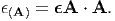 | (3.100) |
This constrained optimization is done by what is called as the Lagrange-multiplier method. Towards this, we introduce the function
![L(A, α *) = A ⋅ ϵA - α*[∥A ∥2 - 1],](main432x.png) | (3.101) |
where α* is the Lagrange multiplier and the condition ∥A∥2 - 1 = 0 characterizes
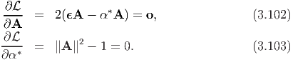
the constraint condition. At locations where the extremal values of  occurs, the
derivatives
occurs, the
derivatives  and
and  must vanish, i.e.,
 a and αa*’s such
that
a and αa*’s such
that
![[ϵ - α *1]Aˆa = o, ∥Aˆa ∥2 = 1,
a](main437x.png) | (3.104) |
(a = 1, 2, 3; no summation) which is nothing but the eigenvalue problem involving the tensor ϵ with the Lagrange multiplier being identified as the eigenvalue. Hence, the results of section 2.5 follows. In particular, for (3.104a) to have a non-trivial solution
 | (3.105) |
where
![1- 2 2
I1 = tr(ϵ), I2 = 2[I1 - tr(ϵ )], I3 = det(ϵ),](main439x.png) | (3.106) |
the principal invariants of the strain ϵ. As stated in section 2.5, equation (3.105 has three real roots, since the linearized strain tensor is symmetric. These roots (αa*) will henceforth be denoted by ϵ 1, ϵ2 and ϵ3 and are called principal strains. The principal strains include both the maximum and minimum normal strains among all material fibers passing through a given x.
The corresponding three orthonormal eigenvectors  a, which are then
characterized through the relation (3.104) are called the principal directions of ϵ.
Further, these eigenvectors form a mutually orthogonal basis since the strain
tensor ϵ is symmetric. This property of the strain tensor also allows us to
represent ϵ in the spectral form
a, which are then
characterized through the relation (3.104) are called the principal directions of ϵ.
Further, these eigenvectors form a mutually orthogonal basis since the strain
tensor ϵ is symmetric. This property of the strain tensor also allows us to
represent ϵ in the spectral form
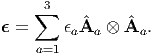 | (3.107) |
As we did to obtain equation (3.89) when the components of the displacement gradient are small, the right Cauchy-Green deformation tensor could be approximately computed as, C ≈ 1 + 2ϵ. For this approximation, the deformed angle between two line segments initially oriented along A1 and A2 directions given in (3.66) simplifies to,
 | (3.108) |
where we have approximated (1 + 2ϵA ⋅ A) as 1, since the components of ϵ is much less than 1 (of the order of 10-3) and the components of A is less than or equal to 1. If α is the angle between the line elements in the reference configuration, then cos(α) = A1 ⋅ A2. Using the trigonometric relation, cos(A) - cos(B) = 2 sin((A + B)∕2) sin((B - A)∕2) and the assumption that the change in angle, αf - α, is small, equation (3.108) could be written as,
 | (3.109) |
When A1 and A2 are identified with the orthonormal coordinate basis, then sin(α) = 1 and ϵA1 ⋅ A2 represents the off diagonal terms in the matrix representation of the components of the strain tensor. Hence, the off diagonal terms are the shear strains which represents half of the change in angle between orthogonal line elements oriented along the coordinate basis directions.
Therefore, we conclude that the diagonal elements in the matrix representation of the components of the strain tensor are related to the changes in length of line elements oriented along the direction of the orthonormal coordinate basis and the off diagonal elements are related to the changes in angle of these line elements oriented along the direction of the orthonormal basis. We also infer that there is no change in angle between line elements along which the change in length is a extremum. This is a consequence of the observation that the off diagonal elements are zero in the equation (3.107) representing the strain using the principal directions as the coordinate basis.
Now, we are interested in finding how the components of the linearized strain
change due to transformation of the coordinate basis. By virtue of the linearized
strain being a second order tensor, the transformation laws (2.161) derived in
section 2.6.2 hold. Thus, if Qij (= ei ⋅ j) represents the directional cosine
matrix of the transformation from coordinate basis {e1,e2,e3} to the
basis {
j) represents the directional cosine
matrix of the transformation from coordinate basis {e1,e2,e3} to the
basis { 1,
1, 2,
2, 3}, then the strain components in the
  i basis,
  ij could be
obtained from the strain components in the ei basis, ϵij, through the
equation,
ij could be
obtained from the strain components in the ei basis, ϵij, through the
equation,
 | (3.110) |
Let us specialize to a state of strain wherein the strain tensor has a representation,
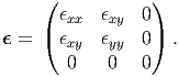 | (3.111) |
This state of strain is called as plane strain. A state of strain is said to be plane
strain if at least one of its principal values is zero which means that det(ϵ) = 0.
Let us further assume that  j is related to ei through,
 | (3.112) |
This represents a anticlockwise rotation of the ei basis about e3 basis to obtain the new basis vectors (see figure 3.7). Substituting equations (3.111) and (3.112) in (3.110) we obtain,
![2 2
˜ϵxx = ϵxx cos (θ) + ϵxy sin(2θ) + ϵyy sin (θ)
[ϵxx + ϵyy] [ϵxx - ϵyy]
= ----------+ ---------- cos(2θ) + ϵxy sin(2θ),
2 2](main455x.png) | (3.113) |
![2 2
˜ϵxy = - ϵxx sin(θ) cos(θ) + ϵxy[cos (θ) - sin (θ)] + ϵyy sin(θ)cos(θ)
[ϵxx - ϵyy]
= - ---------- sin(2θ) - ϵxy cos(2θ),
2](main456x.png) | (3.114) |
![2 2
˜ϵyy = ϵxx sin (θ) - ϵxy sin(2θ) + ϵyy cos (θ )
[ϵxx + ϵyy] [ϵxx - ϵyy]
= ----------- ----------cos(2θ) - ϵxy sin (2θ).
2 2](main457x.png) | (3.115) |
Let us now understand what we mean when we say the motion to be homogeneous. Say, in the reference configuration, we have marked straight lines with different slopes on each of the three mutually perpendicular planes (material curves). Even, if only some of the line segments transform into curves the motion is inhomogeneous. Examples of such motions are plenty. A beam subjected to a pure bending moment6 is an example. Thus, we can show that for a homogeneous motion the matrix components of the deformation gradient, F with respect to a Cartesian basis can depend only on time and hence any homogeneous motion can be written in the form:
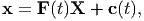 | (3.116) |
where c is some vector which depends on time, X and x are the position vectors of the same material particle in the reference and current configuration, respectively.
Recognize that, in general, the matrix components of the deformation gradient, F with respect to a curvilinear basis (say cylindrical polar basis) need not be a constant for the deformation to be homogeneous nor would the deformation be homogeneous if the matrix components with respect to a curvilinear basis were to be a constant. For example, consider a deformation of the form:
 |
where
An example, of homogeneous motion is rigid body motion. Here apart from straight lines deforming into straight lines, the distance between any two points in the body remain the same. Let X1 and X2 be the position vectors of two material points in the reference configuration and let the position vector of the same material particle in the current configuration be denoted by x1 and x2, then, if the body undergoes rigid body motion:
 | (3.117) |
Since, this motion is homogeneous
 | (3.118) |
Combining equations (3.117) and (3.118) we obtain
 | (3.119) |
Since X1 ≠ X2 and (3.119) has to hold for any pair of material particles, i.e., X1 and X2 are some arbitrary but distinct vectors, we require that
 | (3.120) |
for a rigid body motion. Recalling the definition of an orthogonal tensor, (2.92) and comparing it with (3.120), we immediately recognize that for a rigid body motion, the deformation gradient has to be an orthogonal tensor.
For example, consider, a motion given by
![x = Q (t)[X - Xo] + c(t),](main465x.png) | (3.121) |
where Q is an orthogonal tensor which is a function of time, Xo is a constant vector and c is a vector function of time.
Straight forward computation from the definition of the various quantities would show that the deformation gradient, F, the right and left Cauchy-Green deformation tensors, C and B respectively, the Cauchy-Green strain tensor, E and the Almansi-Hamel strain tensor, e for this rigid body deformation are,
 |
The Lagrangian displacement gradient, H and the Eulerian displacement gradient, h are:
 |
then, the Lagrangian linearized strain tensor, ϵL and the Eulerian linearized strain tensor, ϵE are evaluated to be,
![ϵL = 1[Q + Qt - 21], ϵE = 1[21 - Q - Qt],
2 2](main468x.png) |
Observe that the given motion corresponds to rigid body rotation of the body about Xo and a translation. For this motion, we expect the strains to be zero because the length between two points do not change in a rigid body deformation. While the Cauchy-Green strain tensor and Almansi-Hamel strain tensor meets these requirements the linearized strain tensors don’t. However, recognize that these measures are valid only for cases when tr(HHt) = tr(hht) = tr(21 - Q - Qt) << 1. That is to use linearized strain measures the rigid body rotation has to be small. Hence, linearized strain measures can be used only when the change in length is small and the angle of rotation of the line segment is small too.
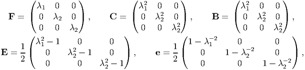
An uniaxial or equi-biaxial motion has the form:
 | (3.122) |
where λ1 and λ2 are functions of time and (X,Y,Z) denotes the Cartesian coordinates of a typical material particle in the reference configuration and (x,y,z) denote the Cartesian coordinates of the same material particle in the current configuration. If this motion is effected by the application of the force (traction) along just one direction (in this case along ex), then it is called uniaxial motion. On the other hand if the deformation is effected by the application of force along two directions(in this case along ey and ez), then it is called equi-biaxial motion.
For the assumed motion field (3.122), the deformation gradient, F, the right and left Cauchy-Green deformation tensors, C and B respectively, the Cauchy-Green strain tensor, E and the Almansi-Hamel strain tensor, e are computed to be,
 |
 |
then, the Lagrangian linearized strain tensor, ϵL and the Eulerian linearized strain tensor, ϵE are evaluated to be,
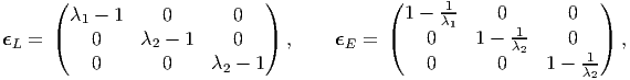 |
Though the form of the Cauchy-Green, Almansi-Hamel, Lagrangian linearized and Eulerian linearized strain look different it can be easily verified that when λi is close to 1, numerically their values would also be close to each other.
Now, say a unit cube oriented in space such that =
{(X,Y,Z)|0 ≤ X ≤ 1, 0 ≤ Y ≤ 1, 0 ≤ Z ≤ 1} is subjected to a deformation of the
form (3.122). Then, the deformed volume of the cube, v as given by (3.75) is v =
det(F) = λ1λ22. Notice that the cube being of unit dimensions its original volume
is 1. Similarly, the deformed surface area, a of the face whose normal coincides
with ex in the reference configuration is computed from (3.74) as, a =
det(F)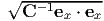 = λ22 and the deformed normal direction is found using
Nanson’s formula (3.72) as, n = det(F)F-te
x(1∕a) = ex. The deformed length of
a line element oriented along (ex + ey)∕
= λ22 and the deformed normal direction is found using
Nanson’s formula (3.72) as, n = det(F)F-te
x(1∕a) = ex. The deformed length of
a line element oriented along (ex + ey)∕ and of unit length is
  obtained by using (3.60). Similarly, the deformed angle between line segments
oriented along ex and (ex + ey)∕
obtained by using (3.60). Similarly, the deformed angle between line segments
oriented along ex and (ex + ey)∕ is, αf = cos -1(λ
1∕
is, αf = cos -1(λ
1∕ ) which is found
using (3.66).
) which is found
using (3.66).
Motions in which the volume of a body does not change are called isochoric motions. Thus it follows from (3.75) that det(F) = 1 for these motions. In case of motions for which the magnitude of the components of the displacement gradient are small, then det(F) can be approximately computed as 1 + tr(ϵ) and thus for this deformation to be isochoric it suffices if tr(ϵ) = 0. Isochoric motion can be homogeneous or inhomogeneous. However, the examples that we shall consider here are homogeneous motions.
An isochoric uniaxial or equi-biaxial motion takes the form:
 | (3.123) |
where λ is a function of time and as before (X,Y,Z) denotes the Cartesian coordinates of a typical material particle in the reference configuration and (x,y,z) denote the Cartesian coordinates of the same material particle in the current configuration. It is easy to check that det(F) for this deformation is 1.
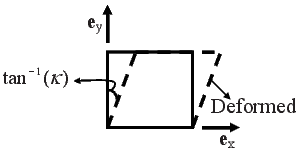
A simple shear motion has the form:
 | (3.124) |
where κ is only a function of time. It is easy to verify that this motion is isochoric. In this case, the body is assumed to shear in the X - Y plane that is the angle between line segments initially oriented along the ex and ey direction change (see figure 3.8) but the angle between line segments initially oriented along ey and ez direction or ez and ex direction does not change.
For the pure shear motion field (3.124), the deformation gradient, F, the right and left Cauchy-Green deformation tensors, C and B respectively, the Cauchy-Green strain tensor, E and the Almansi-Hamel strain tensor, e are computed to be,
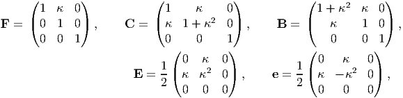 |
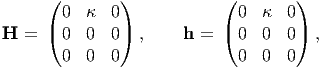 |
then, the Lagrangian linearized strain tensor, ϵL and the Eulerian linearized strain tensor, ϵE are evaluated to be,
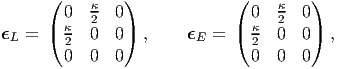 |
It can be seen from the above that while the Cauchy-Green and Almansi-Hamel tells that the length of line segments along the ey direction would change apart from a change in angle of line segments oriented along the ex and ey directions, Lagrangian linearized and Eulerian linearized strain does not tell that the length of the line segments along ey changes. This is because, the change in length along the ey direction is of order κ2, terms that we neglected to obtain linearized strain. Careful experiments on steel wires of circular cross section subjected to torsion7 shows axial elongation, akin to the development of the normal strain along ey direction. It is this observation that proved that linearized strain is an approximation of the actual strain.
Now, say a unit cube oriented in space such that =
{(X,Y,Z)|0 ≤ X ≤ 1, 0 ≤ Y ≤ 1, 0 ≤ Z ≤ 1} is subjected to a deformation of the
form (3.124). Then, the deformed volume of the cube, v as given by (3.75) is v =
det(F) = 1. Similarly, the deformed surface area, a of the face whose
normal coincides with ex in the reference configuration is computed from
(3.74) as, a = det(F) = 1 + κ2 and the deformed normal
direction is found using Nanson’s formula (3.72) as, n = det(F)F-te
x(1∕a)
= [ex - κey]∕[1 + κ2]. The deformed length of a line element oriented
along (ex + ey)∕
= 1 + κ2 and the deformed normal
direction is found using Nanson’s formula (3.72) as, n = det(F)F-te
x(1∕a)
= [ex - κey]∕[1 + κ2]. The deformed length of a line element oriented
along (ex + ey)∕ and of unit length is
  obtained by
using (3.60). Similarly, the deformed angle between line segments oriented
along ex and (ex + ey)∕
obtained by
using (3.60). Similarly, the deformed angle between line segments oriented
along ex and (ex + ey)∕ is, αf = cos -1([1 + κ]∕
 ) which
is found using (3.66). In the above computations we have not assumed
that the value of κ is small; if we do the final expressions would be much
simpler.
) which
is found using (3.66). In the above computations we have not assumed
that the value of κ is small; if we do the final expressions would be much
simpler.
Till now we studied on ways to find the strain given a displacement field.
However, there arises a need while solving boundary value problems wherein we
would need to find the displacement given the strain field. This problem involves
finding the 3 components of the displacement from the 6 independent components
of the strain (only six components since strain is a symmetric tensor) that has
been prescribed. To be able to find a continuous displacement field from the
prescribed 6 components of the linearized strain, all these 6 components cannot be
prescribed arbitrarily. The restrictions that these prescribed 6 components of the
strain should satisfy is given by the compatibility condition. These restrictions are
obtained from the requirement that the sequence of differentiation is immaterial
when the first derivative of the multivariate function is continuous, i.e.,  =
=
 . Working with index notation, the Cartesian components of the linearized
strain is,
. Working with index notation, the Cartesian components of the linearized
strain is,
![[ ]
1- ∂ui- ∂uj-
ϵij = 2 ∂xj + ∂xi ,](main491x.png) | (3.125) |
where ui are the Cartesian components of the displacement vector, xi are the Cartesian coordinates of a point. Then, computing
![∂2ϵij 1 [ ∂3ui ∂uj ]
------- = -- -----------+ ---------- , (3.126)
∂xk ∂xl 2 [∂xk ∂xl∂xj ∂xk ∂xl∂xi]
-∂2ϵkl- 1- ---∂3uk--- ----∂ul----
∂x ∂x = 2 ∂x ∂x ∂x + ∂x ∂x ∂x , (3.127)
i2 j [ i3 j l i j k ]
-∂-ϵjl- = 1- ---∂-uj--- + ----∂ul---- , (3.128)
∂xi∂xk 2 ∂xi∂xk ∂xl ∂xi∂xk ∂xj
2 [ 3 ]
-∂-ϵik- = 1- ---∂-ui----+ ----∂uk--- , (3.129)
∂xj ∂xl 2 ∂xj∂xl ∂xk ∂xj ∂xl∂xi](main492x.png)
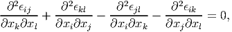 | (3.130) |
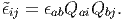
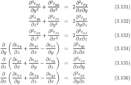
since the order of differentiation is immaterial. Equation (3.130) is called Saint Venant compatibility equations. It can be also seen that equation (3.130) has 81 individual equations as each of the index - i, j, k, l - takes values 1, 2 and 3. It has been shown that of these 81 equations most are either simple identities or repetitions and only 6 are meaningful. These six equations involving the 6 independent Cartesian components of the linearized strain are:
Next, we show that these 6 equations are necessary conditions. For this assume ϵxy = xy and all other component of the strains are 0. For this strain it can be shown that equation (3.131) alone is violated and that no smooth displacement field would result in this state of strain. Similarly, on assuming
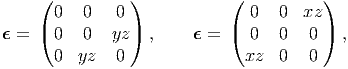 |
we find that for each of these state of strain only one of the compatibility equations is violated; equation (3.132) for the first strain and (3.133) for the other strain. In the same fashion, on assuming
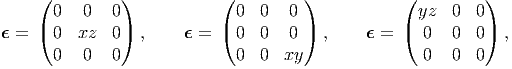 |
we find that for each of these state of strain only one of the compatibility equations is violated; equation (3.134) for the first strain, (3.135) for the second strain and (3.136) for the last strain. Thus, we find that all the six equations are required to ensure the existence of a smooth displacement field given a strain field.
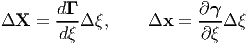
However, there are claims that the number of independent compatibility equations is only three. This is not correct for the following reasons. On differentiating the strain field four times instead of twice as done in case of compatibility condition, the six compatibility equations (3.131) through (3.136) can be shown to be equivalent to the following three equations:
This assumes existence of non-zero higher derivatives of strain field which may not be always true, as in the case of the strain field assumed above. Hence, only if higher order derivatives of strain field exist and is different from zero can one replace the 6 compatibility conditions (3.131) through (3.136) by (3.137) through (3.139).Further, it is not easy to show that the above compatibility conditions (3.131) through (3.136) are sufficient to find a smooth displacement field given a strain field (see for example Sadd [4] to establish sufficiency of these conditions). In fact the sufficiency of these conditions in multiply connected8 bodies is yet to be established.
It should be mentioned that the form of the compatibility equation depends on the strain measure that is prescribed. For Cauchy-Green strain it is given in terms of the Riemannian tensor for simply connected bodies9 . However, it is still not clear what these compatibility conditions have to be for other classes of bodies when Cauchy-Green strain is used. Development of compatibility conditions for other strain measures is beyond the scope of this course.
In this chapter, we saw how to describe the motion of a body. Then, we focused on finding how curves, surfaces and volumes get transformed due to this motion. These transformations seem to depend on right Cauchy-Green deformation tensor, C, related to the gradient of the deformation field, F through
 | (3.140) |
This was followed by a discussion on a need for a quantity called strain and various definitions of the strain. Associated with each definition of strain, we found a strain tensor that carried all the information required to compute the strain along any direction. Here we showed that when the components of the gradient of the displacement field, h, is small then the term hth in the definition of the strain can be ignored to obtain, what is called as the linearized strain tensor,
![1- t
ϵ = 2 [h + h ].](main499x.png) | (3.141) |
By virtue of the linearized strain being symmetric, there are only 6 independent components. Since, these 6 independent components are to be obtained from a smooth displacement field, they cannot be prescribed arbitrarily. It was shown that they have to satisfy the compatibility condition.
This completes our study on the motion of bodies. Since, in this course, we are interested in understanding the response of solid like materials undergoing non-dissipative response, we did not study in detail about velocity and its gradients. A course on fluid mechanics would focus on velocity field and its gradient. In the following chapter we shall discuss the concept of stress.
= {(X,Y,Z)|0 ≤ X ≤ 1cm, 0 ≤ Y ≤ 1cm, 0 ≤ Z ≤ 1cm}
in the reference configuration, is subjected to the following deformation
field: x = X, y = Y + A * Z, z = Z + A * Y , where A is a constant
and (X,Y,Z) are the Cartesian coordinates of a material point
before deformation and (x,y,z) are the Cartesian coordinates of the
same material point after deformation. For the specified deformation
field:

Here as usual (X,Y,Z) denotes the coordinates of a typical material particle in the reference configuration and {ei} the Cartesian coordinate basis. For these deformation fields find parts (a) to (l) in problem 1.
=
{(R, Θ,Z)|0.5 ≤ R ≤ 1cm, 0 ≤ Θ ≤ 2π, 0 ≤ Z ≤ 10cm} is subjected to the
following deformation field: r = 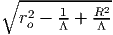 , θ = Θ + ΩZ, z = ΛZ, where
(R, Θ,Z) denote the coordinates of a typical material particle in the
reference configuration, (r,θ,z) denote the coordinates of the same material
particle in the current configuration, ro, Ω and Λ are constants. For this
deformation field:
, θ = Θ + ΩZ, z = ΛZ, where
(R, Θ,Z) denote the coordinates of a typical material particle in the
reference configuration, (r,θ,z) denote the coordinates of the same material
particle in the current configuration, ro, Ω and Λ are constants. For this
deformation field:
 . Assume ro = 1.1, Λ = 1.2 and Ω = 0.1
= {(X,Y,Z)|0 ≤ X ≤ 1, 0 ≤ Y ≤ 1, 0 ≤ Z ≤ 1}
in the reference configuration, is subjected to the following deformation
field: x = X, y = Y + A*X, z = Z, where A is a constant and (X,Y,Z) are
the Cartesian coordinates of a material point before deformation and
(x,y,z) are the Cartesian coordinates of the same material point after
deformation. For the specified deformation field:
= {(X,Y,Z)|0 ≤ X ≤ 1, 0 ≤ Y ≤ 1, 0 ≤ Z ≤ 1}
in the reference configuration, is subjected to the following linearized strain
field:
. Assume ro = 1.1, Λ = 1.2 and Ω = 0.1
= {(X,Y,Z)|0 ≤ X ≤ 1, 0 ≤ Y ≤ 1, 0 ≤ Z ≤ 1}
in the reference configuration, is subjected to the following deformation
field: x = X, y = Y + A*X, z = Z, where A is a constant and (X,Y,Z) are
the Cartesian coordinates of a material point before deformation and
(x,y,z) are the Cartesian coordinates of the same material point after
deformation. For the specified deformation field:
= {(X,Y,Z)|0 ≤ X ≤ 1, 0 ≤ Y ≤ 1, 0 ≤ Z ≤ 1}
in the reference configuration, is subjected to the following linearized strain
field:
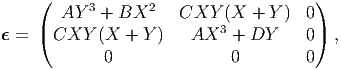 | (3.142) |
where A, B, C, D are constants, find conditions, if any, on the constants if this strain field is to be obtained from a smooth displacement field of the cube. For this value of the constants, find the smooth displacement field that gives raise to the above linearized strain field in a cube. Assume the coordinates of the point (0, 0, 0) after deformation is (10, 0, 0) and that of the point (0, 0, 1) after deformation is (10, 0, 1) to determine the unknown constants in the displacement field. For what magnitude of these constants is the use of linearized strain justified.
 | (3.143) |
For this constant strain field, find
 and of length 1 mm
 and (ex - ey)∕

![4 3 [ ]
-∂-ϵxx-= ---∂---- - ∂-ϵyz + ∂ϵxz+ ∂ϵxy- , (3.137)
∂y2∂z2 ∂x ∂y∂z ∂x ∂y ∂z
4 3 [ ]
-∂--ϵyy- = --∂----- ∂-ϵyz - ∂ϵxz+ ∂ϵxy- , (3.138)
∂z2 ∂x2 ∂x∂y ∂z ∂x ∂y ∂z
∂4ϵzz ∂3 [ ∂ϵyz ∂ϵxz ∂ϵxy]
--2---2 = -------- ----+ ------ ----- . (3.139)
∂x ∂y ∂x ∂y∂z ∂x ∂y ∂z](main497x.png)