In the introduction, we saw that some of the quantities like force is a vector or first order tensor, stress is a second order tensor or simply a tensor. The algebra and calculus associated with these quantities differs, in some aspects from that of scalar quantities. In this chapter, we shall study on how to manipulate equations involving vectors and tensors and how to take derivatives of scalar valued function of a tensor or tensor valued function of a tensor.
A physical quantity, completely described by a single real number, such as temperature, density or mass is called a scalar. A vector is a directed line element in space used to model physical quantities such as force, velocity, acceleration which have both direction and magnitude. The vector could be denoted as v or v. Here we denote vectors as v. The length of the directed line segment is called as the magnitude of the vector and is denoted by |v|. Two vectors are said to be equal if they have the same direction and magnitude. The point that vector is a geometric object, namely a directed line segment cannot be overemphasized. Thus, for us a set of numbers is not a vector.
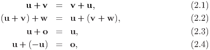
The sum of two vectors yields a new vector, based on the parallelogram law of addition and has the following properties:
Then the scalar multiplication αu produces a new vector with the same direction as u if α > 0 or with the opposite direction to u if α < 0 with the following properties:
The dot (or scalar or inner) product of two vectors u and v denoted by u ⋅ v assigns a real number to a given pair of vectors such that the following properties hold:
 | (2.12) |
A vector e is called a unit vector if |e| = 1. A nonzero vector u is said to be orthogonal (or perpendicular) to a nonzero vector v if: u ⋅ v = 0. Then, the projection of a vector u along the direction of a vector e whose length is unity is given by: u ⋅ e
So far algebra has been presented in symbolic (or direct or absolute) notation. It represents a very convenient and concise tool to manipulate most of the relations used in continuum mechanics. However, particularly in computational mechanics, it is essential to refer vector (and tensor) quantities to a basis. Also, for carrying out mathematical operations more intuitively it is often helpful to refer to components.
We introduce a fixed set of three basis vectors e1, e2, e3 (sometimes introduced as i, j, k) called a Cartesian basis, with properties:
 | (2.13) |
so that any vector in three dimensional space can be written in terms of these three basis vectors with ease. However, in general, it is not required for the basis vectors to be fixed or to satisfy (2.13). Basis vectors that satisfy (2.13) are called as orthonormal basis vectors.
Any vector u in the three dimensional space is represented uniquely by a linear combination of the basis vectors e1, e2, e3, i.e.
 | (2.14) |
where the three real numbers u1, u2, u3 are the uniquely determined Cartesian components of vector u along the given directions e1, e2, e3, respectively. In other words, what we are doing here is representing any directed line segment as a linear combination of three directed line segments. This is akin to representing any real number using the ten arabic numerals.
If an orthonormal basis is used to represent the vector, then the components of the vector along the basis directions is nothing but the projection of the vector on to the basis directions. Thus,
 | (2.15) |
Using index (or subscript or suffix) notation relation (2.14) can be written as u = ∑ i=13 u iei or, in an abbreviated form by leaving out the summation symbol, simply as
 | (2.16) |
where we have adopted the summation convention, invented by Einstein. The summation convention says that whenever an index is repeated (only once) in the same term, then, a summation over the range of this index is implied unless otherwise indicated. The index i that is summed over is said to be a dummy (or summation) index, since a replacement by any other symbol does not affect the value of the sum. An index that is not summed over in a given term is called a free (or live) index. Note that in the same equation an index is either dummy or free. Here we consider only the three dimensional space and denote the basis vectors by {ei}i∈{1,2,3} collectively.
In light of the above, relations (2.13) can be written in a more convenient form as
 | (2.17) |
where δij is called the Kronecker delta. It is easy to deduce the following identities:
 | (2.18) |
The projection of a vector u onto the Cartesian basis vectors, ei yields the ith component of u. Thus, in index notation u ⋅ ei = ui.
As already mentioned a set of numbers is not a vector. However, for ease of computations we represent the components of a vector, u obtained with respect to some basis as,
 | (2.19) |
instead of writing as u = uiei using the summation notation introduced above. The numbers u1, u2 and u3 have no meaning without the basis vectors which are present even though they are not mentioned explicitly.
If ui and vj represents the Cartesian components of vectors u and v respectively, then,
The cross (or vector) product of u and v, denoted by u ∧ v produces a new vector satisfying the following properties:
The cross product characterizes the area of a parallelogram spanned by the vectors u and v given that
 | (2.26) |
where θ is the angle between the vectors u and v and n is a unit vector normal to the plane spanned by u and v, as shown in figure 2.1.
In order to express the cross product in terms of components we introduce the permutation (or alternating or Levi-Civita) symbol ϵijk which is defined as
 | (2.27) |
with the property ϵijk = ϵjki = ϵkij, ϵijk = -ϵikj and ϵijk = -ϵjik, respectively. Thus, for an orthonormal Cartesian basis, {e1,e2,e3}, ei ∧ ej = ϵijkek
It could be verified that ϵijk may be expressed as:
 | (2.28) |
It could also be verified that the product of the permutation symbols ϵijkϵpqr is related to the Kronecker delta by the relation
 | (2.29) |
We deduce from the above equation (2.29) the important relations:
 | (2.30) |
The triple scalar (or box) product: [u,v,w] represents the volume V of a parallelepiped spanned by u, v, w forming a right handed triad. Thus, in index notation:
![V = [u,v,w ] = (u ∧ v) ⋅ w = ϵijkuivjwk.](main55x.png) | (2.31) |
Note that the vectors u, v, w are linearly dependent if and only if their scalar triple product vanishes, i.e., [u,v,w] = 0
The product (u ∧ v) ∧ w is called the vector triple product and it may be verified that
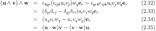
 | (2.36) |
Thus triple product, in general, is not associative, i.e., u ∧ (v ∧ w) ≠ (u ∧ v) ∧ w.
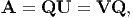
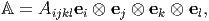
A second order tensor A, for our purposes here, may be thought of as a linear function that maps a directed line segment to another directed line segment. This we write as, v = Au where A is the linear function that assigns a vector v to each vector u. Since A is a linear function,
 | (2.37) |
for all vectors u, v and all scalars α, β.
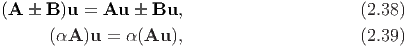
If A and B are two second order tensors, we can define the sum A + B, the difference A - B and the scalar multiplication αA by the rules
If the relation v ⋅ Av ≥ 0 holds for all vectors, then A is said to be a positive semi-definite tensor. If the condition v ⋅ Av > 0 holds for all nonzero vectors v, then A is said to be positive definite tensor. Tensor A is called negative semi-definite if v ⋅ Av ≤ 0 and negative definite if v ⋅ Av < 0 for all vectors, v ≠ o, respectively.
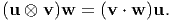
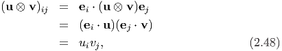
The tensor (or direct or matrix) product or the dyad of the vectors u and v is denoted by u ⊗ v. It is a second order tensor which linearly transforms a vector w into a vector with the direction of u following the rule
 | (2.40) |
The dyad satisfies the linearity property
 | (2.41) |
The following relations are easy to establish:
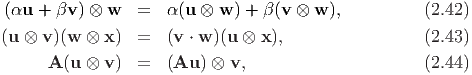
A dyadic is a linear combination of dyads with scalar coefficients, for example, α(u ⊗ v) + β(w ⊗ x). Any second-order tensor can be expressed as a dyadic. As an example, the second order tensor A may be represented by a linear combination of dyads formed by the Cartesian basis {ei}, i.e., A = Aijei ⊗ ej. The nine Cartesian components of A with respect to {ei}, represented by Aij can be expressed as a matrix [A], i.e.,
![⌊ ⌋
A11 A12 A13
[A ] = ⌈ A21 A22 A23 ⌉.
A31 A32 A33](main63x.png) | (2.45) |
This is known as the matrix notation of tensor A. We call A, which is resolved along basis vectors that are orthonormal and fixed, a Cartesian tensor of order two. Then, the components of A with respect to a fixed, orthonormal basis vectors ei is obtained as:
 | (2.46) |
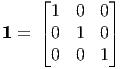
The Cartesian components of the unit tensor 1 form the Kronecker delta symbol, thus 1 = δijei ⊗ ej = ei ⊗ ei and in matrix form
 | (2.47) |
Next we would like to derive the components of u ⊗ v along an orthonormal basis {ei}. Using the representation (2.46) we find that
![⌊ ⌋ ⌊ ⌋
u1 [ ] u1v1 u1v2 u1v3
(u ⊗ v)ij = ⌈ u2 ⌉ v1 v2 v3 = ⌈ u2v1 u2v2 u2v3 ⌉.
u3 u3v1 u3v2 u3v3](main67x.png) | (2.49) |
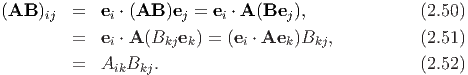
The product of two second order tensors A and B, denoted by AB, is again a second order tensor. It follows from the requirement (AB)u = A(Bu), for all vectors u.
Further, the product of second order tensors is not commutative, i.e., AB ≠ BA. The components of the product AB along an orthonormal basis {ei} is found to be:
The following properties hold for second order tensors:
Note that the relations AB = 0 and Au = o does not imply that A or B is 0 or u = o.
The unique transpose of a second order tensor A denoted by At is governed by the identity:
 | (2.60) |
for all vectors u and v.
Some useful properties of the transpose are
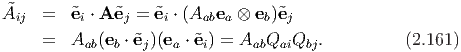
From identity (2.60) we obtain ei ⋅ Ate j = ej ⋅ Aei, which gives, in regard to equation (2.46), the relation (At) ij = Aji.
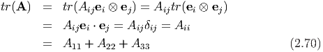
The trace of a tensor A is a scalar denoted by tr(A) and is defined as:
![tr(A ) = [Au,--v,w-] +-[u,Av,-w-] +-[u,v,Aw-]-
[u,v, w ]](main72x.png) | (2.65) |
where u, v, w are any vectors such that [u,v,w] ≠ 0, i.e., these vectors span the entire 3D vector space. Thus, tr(m ⊗ n) = m ⋅ n. Let us see how: Without loss of generality we can assume the vectors u, v and w to be m, n and (m ∧ n) respectively. Then, (2.65) becomes
![(n ⋅ m )[m, n, m ∧ n ] + |n|[m, m, m ∧ n] + [m, n, n][m, n, m ]
tr(m ⊗ n) = -----------------------------------------------------------,
[m, n, m ∧ n]
= n ⋅ m. (2.66)](main73x.png)
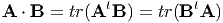
The dot product between two tensors denoted by A ⋅ B, just like the dot product of two vectors yields a real value and is defined as
 | (2.71) |
Next, we record some useful properties of the dot operator:
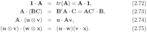
The norm of a tensor A is denoted by |A| (or ∥A∥). It is a non-negative real number and is defined by the square root of A ⋅ A, i.e.,
 | (2.76) |
The determinant of a tensor A is defined as:
![det (A ) = [Au,--Av,-Aw--],
[u,v, w ]](main79x.png) | (2.77) |
where u, v, w are any vectors such that [u,v,w] ≠ 0, i.e., these vectors span the entire 3D vector space. In index notation:
 | (2.78) |
Then, it could be shown that
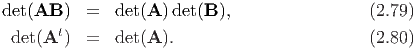
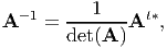
A tensor A is said to be singular if and only if det(A) = 0. If A is a non-singular tensor i.e., det(A) ≠ 0, then there exist a unique tensor A-1, called the inverse of A satisfying the relation
 | (2.81) |
If tensors A and B are invertible (i.e., they are non-singular), then the properties
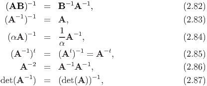
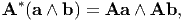
Corresponding to an arbitrary tensor A there is a unique tensor A*, called the adjugate of A, such that
 | (2.88) |
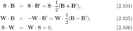
for any arbitrary vectors a and b in the vector space. Suppose that A is invertible and that a, b, c are arbitrary vectors, then
![t* t t t -t
A (a ∧ b) ⋅ c = [A a,A b,A A c ]
= det (At )(a ∧ b) ⋅ {A -tc}
- 1
= det (A ){A (a ∧ b )} ⋅ c, (2.89)](main85x.png)
 | (2.90) |
between the inverse of A and the adjugate of At.
An orthogonal tensor Q is a linear function satisfying the condition
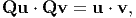 | (2.91) |
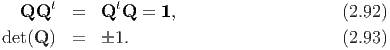
for all vectors u and v. As can be seen, the dot product is invariant (its value does not change) due to the transformation of the vectors by the orthogonal tensor. The dot product being invariant means that both the angle, θ between the vectors u and v and the magnitude of the vectors |u|, |v| are preserved. Consequently, the following properties of orthogonal tensor can be inferred:
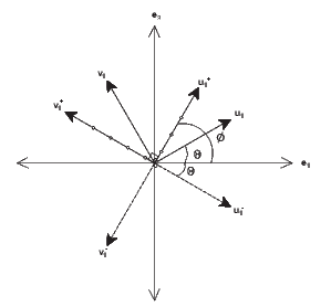
It follows from (2.92) that Q-1 = Qt. If det(Q) = 1, Q is said to be proper orthogonal tensor and this transformation corresponds to a rotation. On the other hand, if det(Q) = -1, Q is said to be improper orthogonal tensor and this transformation corresponds to a reflection superposed on a rotation.Figure 2.2 shows what happens to two directed line segments, u1 and v1 under the action the two kinds of orthogonal tensors. A proper orthogonal tensor corresponding to a rotation about the e3 basis, whose Cartesian coordinate components are given by
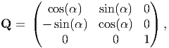 | (2.94) |
transforms, u1 to u1+ and v 1 to v1+, maintaining their lengths and the angle between these line segments. Here α = Φ - Θ. An improper orthogonal tensor corresponding to reflection about e1 axis, whose Cartesian coordinate components are given by
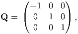 | (2.95) |
transforms, u1 to u1- and v 1 to v1-, still maintaining their lengths and the angle between these line segments a constant.
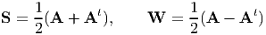
A symmetric tensor, S and a skew symmetric tensor, W are such:
 | (2.96) |
therefore the matrix components of these tensor reads
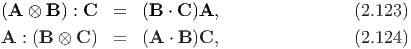
![⌊ S S S ⌋ ⌊ 0 W W ⌋
11 12 13 12 13
[S] = ⌈ S12 S22 S23 ⌉ , [W ] = ⌈ - W12 0 W23 ⌉ ,
S13 S23 S33 - W13 - W23 0](main93x.png) | (2.97) |
thus, there are only six independent components in symmetric tensors and three independent components in skew tensors. Since, there are only three independent scalar quantities that in a skew tensor, it behaves like a vector with three components. Indeed, the relation holds:
 | (2.98) |
where u is any vector and ω characterizes the axial (or dual) vector of the
skew tensor W, with the property |ω| = |W|∕ (proof is omitted). The
relation between the Cartesian components of W and ω is obtained as:
(proof is omitted). The
relation between the Cartesian components of W and ω is obtained as:
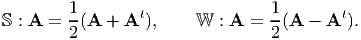
Any tensor A can always be uniquely decomposed into a symmetric tensor, denoted by S (or sym(A)), and a skew (or antisymmetric) tensor, denoted by W (or skew(A)). Hence, A = S + W, where
 | (2.103) |
Next, we shall look at some properties of symmetric and skew tensors:
where B denotes any second order tensor. The first of these equalities in the above equations is due to the property of the dot and trace operator, namely A ⋅ B = At ⋅ Bt and that A ⋅ B = B ⋅ A.
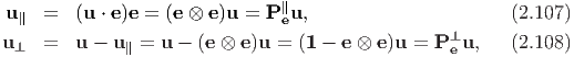
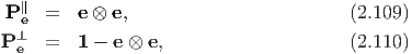
Consider any vector u and a unit vector e. Then, we write u = u∥ + u⊥, with u∥ and u⊥ characterizing the projection of u onto the line spanned by e and onto the plane normal to e respectively. Using the definition of a tensor product (2.40) we deduce that
Any tensor of the form α1, with α denoting a scalar is known as a spherical tensor.
Every tensor A can be decomposed into its so called spherical part and its deviatoric part, i.e.,
![A = α1 + dev (A ), or A = α δ + [dev (A)] ,
ij ij ij](main103x.png) | (2.115) |
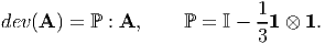
where α = tr(A)∕3 = Aii∕3 and dev(A) is known as a deviator of A or a deviatoric tensor and is defined as dev(A) = A - (1∕3)tr(A)1, or [dev(A)]ij = Aij - (1∕3)Akkδij. It then can be easily verified that tr(dev(A)) = 0, for any second order tensor A.
Above we saw two additive decompositions of an arbitrary tensor A. Of comparable significance in continuum mechanics are the multiplicative decompositions afforded by the polar decomposition theorem. This result states that an arbitrary invertible tensor A can be uniquely expressed in the forms
 | (2.116) |
where Q is an orthogonal tensor and U, V are positive definite symmetric tensors. It should be noted that Q is proper or improper orthogonal according as det(A) is positive or negative. (See, for example, Chadwick [1] for proof of the theorem.)
A fourth order tensor A may be thought of as a linear function that maps second order tensor A into another second order tensor B. While this is too narrow a viewpoint1 , it suffices for the study of mechanics. We write B = A : A which defines a linear transformation that assigns a second order tensor B to each second order tensor A.
We can express any fourth order tensor, A in terms of the three Cartesian basis vectors as
 | (2.117) |
where Aijkl are the Cartesian components of A. Thus, the fourth order tensor A has 34 = 81 components. Remember that any repeated index has to be summed from one through three.
One example for a fourth order tensor is the tensor product of the four vectors u, v, w, x, denoted by u ⊗ v ⊗ w ⊗ x. We have the useful property:
 | (2.118) |
If A = u ⊗ v ⊗ w ⊗ x, then it is easy to see that the Cartesian components of A, Aijkl = uivjwkxl, where ui, vj, wk, xl are the Cartesian components of the vectors u, v, w and x respectively.
Another example of a fourth order tensor, is the tensor obtained from the tensor product of two second order tensors, i.e., D = A ⊗ B, where A, B are second order tensors and D is the fourth order tensor. In index notation we may write: Dijkl = AijBkl where Dijkl, Aij, Bkl are the Cartesian components of the respective tensors.
The double contraction of a fourth order tensor A with a second order tensor B results in a second order tensor, denoted by A : B with the property that:

 | (2.121) |
Next, we compute the Cartesian components of A : B to be:
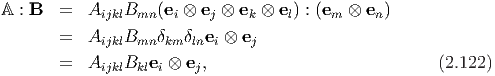
Then, the following can be established:
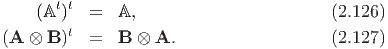
The unique transpose of a fourth order tensor A denoted by At is governed by the identity
 | (2.125) |
for all the second order tensors B and C. From the above identity we deduce the index relation (At) ijkl = Aklij. The following properties of fourth order tensors can be established:
Next, we define fourth order unit tensors I and so that
 | (2.128) |
for any second order tensor A. These fourth order unit tensors may be represented by

The deviatoric part of a second order tensor A may be described by means of a fourth order projection tensor, ℙ where
 | (2.131) |
Thus the components of dev(A) and A are related through the expression [dev(A)]ij = PijklAkl, with Pijkl = δikδjl - (1∕3)δijδkl.
Similarly, the fourth order tensors S and W given by
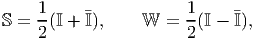 | (2.132) |
are such that for any second order tensor A, they assign symmetric and skew part of A respectively, i.e.,
 | (2.133) |
Till now, we represented second order tensor components in a matrix form, for the advantages that it offers in computing other quantities and defining other operators. However, when we want to study mapping of second order tensor on to another second order tensor, this representation seem to be inconvenient. For this purpose, we introduce this alternate representation. Now, we view the second order tensor as a column vector of nine components instead of a 3 by 3 matrix as introduced in (2.45). The order of these components is subjective. Keeping in mind the application of this is to study elasticity, we order the components of a general second order tensor, A, as,
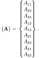 | (2.134) |
In view of this, the fourth order tensor, which for us is a linear function that maps a second order tensor to another second order tensor, can be represented as a 9 by 9 matrix as,
![9
∑
{B }i = [ℂ]ij{A }j, i = 1...9.
j=1](main119x.png) | (2.135) |
where A and B are second order tensors and ℂ is a fourth order tensor. Note that as before the fourth order tensor has 81 (=9*9) components. Thus, now the fourth order tensor is a matrix which is the reason for representing the second order tensor as vector.
The scalar λi characterize eigenvalues (or principal values) of a tensor A if there
exist corresponding nonzero normalized eigenvectors  i (or principal directions or
principal axes) of A, so that
i (or principal directions or
principal axes) of A, so that
 | (2.136) |
To identify the eigenvectors of a tensor, we use subsequently a hat on the vector
quantity concerned, for example,  .
.
Thus, a set of homogeneous algebraic equations for the unknown eigenvalues
λi, i = 1,2,3, and the unknown eigenvectors  i, i = 1,2,3, is
 | (2.137) |
For the above system to have a solution  i ≠ o the determinant of the system
must vanish. Thus,
i ≠ o the determinant of the system
must vanish. Thus,
 | (2.138) |
where
 | (2.139) |
This requires that we solve a cubic equation in λ, usually written as
 | (2.140) |
called the characteristic polynomial (or equation) for A, the solutions of which are the eigenvalues λi, i = 1,2,3. Here, Ii, i = 1,2,3, are the so-called principal scalar invariants of A and are given by
![I1 = tr(A ) = Aii = λ1 + λ2 + λ3,
1 1
I2 = -[(tr(A ))2 - tr(A2 )] = -(AiiAjj - AmnAnm ) = λ1 λ2 + λ2 λ3 + λ1λ3,
2 2
I3 = det(A ) = ϵijkAi1Aj2Ak3 = λ1 λ2λ3. (2.141)](main129x.png)
A repeated application of tensor A to equation (2.136) yields Aα i = λiα
 i, i
= 1,2,3, for any positive integer α. (If A is invertible then α can be any integer;
not necessarily positive.) Using this relation and (2.140) multiplied by
i, i
= 1,2,3, for any positive integer α. (If A is invertible then α can be any integer;
not necessarily positive.) Using this relation and (2.140) multiplied by  i, we
obtain the well-known Cayley-Hamilton equation:
i, we
obtain the well-known Cayley-Hamilton equation:
 | (2.142) |
It states that every second order tensor A satisfies its own characteristic equation. As a consequence of Cayley-Hamilton equation, we can express Aα in terms of A2, A, 1 and principal invariants for positive integer, α > 2. (If A is invertible, the above holds for any integer value of α positive or negative provided α ≠ {0, 1, 2}.)
For a symmetric tensor S the characteristic equation (2.140) always has three
real solutions and the set of eigenvectors form a orthonormal basis { } (the proof
of this statement is omitted). Hence, for a positive definite symmetric tensor A,
all eigenvalues λi are (real and) positive since, using (2.136), we have λi =
} (the proof
of this statement is omitted). Hence, for a positive definite symmetric tensor A,
all eigenvalues λi are (real and) positive since, using (2.136), we have λi =  i ⋅A
i ⋅A i
> 0, i = 1,2,3.
i
> 0, i = 1,2,3.
Any symmetric tensor S may be represented by its eigenvalues λi, i = 1,2,3,
and the corresponding eigenvectors of S forming an orthonormal basis { i}. Thus,
S can be expressed as
i}. Thus,
S can be expressed as
 | (2.143) |
called the spectral representation (or spectral decomposition) of S. Thus, when orthonormal eigenvectors are used as the Cartesian basis to represent S then
![⌊ λ 0 0 ⌋
⌈ 1 ⌉
[S] = 0 λ2 0 .
0 0 λ3](main139x.png) | (2.144) |
The above holds when all the three eigenvalues are distinct. On the other hand, if
there exists a pair of equal roots, i.e., λ1 = λ2 = λ ≠ λ3, with an unique
eigenvector  3 associated with λ3, we deduce that
![∥ ⊥
S = λ3 (nˆ3 ⊗ ˆn3) + λ[1 - (nˆ3 ⊗ ˆn3)] = λ3P ˆn3 + λP ˆn3,](main141x.png) | (2.145) |
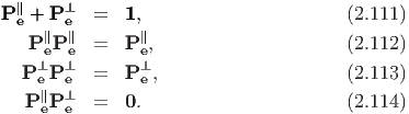
where P 3∥ and P
 3⊥ denote projection tensors introduced in (2.109) and (2.110)
respectively. Finally, if all the three eigenvalues are equal, i.e., λ1 = λ2 = λ3 = λ,
then
3⊥ denote projection tensors introduced in (2.109) and (2.110)
respectively. Finally, if all the three eigenvalues are equal, i.e., λ1 = λ2 = λ3 = λ,
then
 | (2.146) |
where every direction is a principal direction and every set of mutually orthogonal basis denotes principal axes.
It is important to recognize that eigenvalues characterize the physical nature of the tensor and that they do not depend on the coordinates chosen.
Let C be symmetric and positive definite tensor. Then there is a unique positive definite, symmetric tensor U such that
 | (2.147) |
We write  for U. If spectral representation of C is:
 | (2.148) |
then the spectral representation for U is:
 | (2.149) |
where we have assumed that the eigenvalues of C, λi are distinct. On the other hand if λ1 = λ2 = λ3 = λ then
 | (2.150) |
If λ1 = λ2 = λ ≠ λ3, with an unique eigenvector  3 associated with λ3
then
3 associated with λ3
then
![∘ --- √ --
U = λ3(ˆn3 ⊗ ˆn3) + λ[1 - (ˆn3 ⊗ ˆn3)]](main151x.png) | (2.151) |
(For proof of this theorem, see for example, Gurtin [2].)
Consider two sets of mutually orthogonal basis vectors which share a common
origin. They correspond to a ‘new’ and an ‘old’ (original) Cartesian coordinate
system which we assume to be right-handed characterized by two sets of basis
vectors { i} and {ei}, respectively. Hence, the new coordinate system could
be obtained from the original one by a rotation of the basis vectors ei
about their origin. We then define the directional cosine matrix, Qij,
as,
i} and {ei}, respectively. Hence, the new coordinate system could
be obtained from the original one by a rotation of the basis vectors ei
about their origin. We then define the directional cosine matrix, Qij,
as,
 | (2.152) |
Note that the first index on Qij indicates the ‘old’ components whereas the second index holds for the ‘new’ components.
It is worthwhile to mention that vectors and tensors themselves remain invariant upon a change of basis - they are said to be independent of the coordinate system. However, their respective components do depend upon the coordinate system introduced. This is the reason why a set of numbers arranged as a 3 by 1 or 3 by 3 matrix is not a vector or a tensor.
Consider some vector u represented using the two sets of basis vectors {ei} and
{ i}, i.e.,

 | (2.154) |
from the definition of the directional cosine matrix, (2.152). We assume that the
relation between the basis vectors ei and  j is known and hence given the
components of a vector in a basis, its components in another basis can be found
using equation (2.154).
j is known and hence given the
components of a vector in a basis, its components in another basis can be found
using equation (2.154).
In an analogous manner, we find that
 | (2.155) |
The results of equations (2.154) and (2.155) could be cast in matrix notation as
![[u˜] = [Q ]t[u], and [u ] = [Q ][˜u ],](main159x.png) | (2.156) |
respectively. It is important to emphasize that the above equations are not
identical to  = Qtu and u = Q
 , respectively. In (2.156) [
 ] and [u]
are column vectors characterizing components of the same vector in two
different coordinate systems, whereas
] and [u]
are column vectors characterizing components of the same vector in two
different coordinate systems, whereas  and u are different vectors, in the
later. Similarly, [Q] is a matrix of directional cosines, it is not a tensor
even though it has the attributes of an orthogonal tensor as we will see
next.
and u are different vectors, in the
later. Similarly, [Q] is a matrix of directional cosines, it is not a tensor
even though it has the attributes of an orthogonal tensor as we will see
next.
Combining equations (2.154) and (2.155), we obtain
 | (2.157) |
Hence, (QaiQji -δja)ua = 0 and (QijQia -δja)ũa = 0 for any vector u. Therefore,
![Q Q = δ , or [Q ][Q ]t = [1], (2.158)
ai ji ja
QiaQij = δja, or [Q ]t[Q ] = [1]. (2.159)](main165x.png)
To determine the transformation laws for the Cartesian components of any second-order tensor A, we proceed along the lines similar to that done for vectors. Since, we seek the components of the same tensor in two different basis,
 | (2.160) |
Then it follows from (2.46) that,
In matrix notation, [ ] = [Q]t[A][Q]. In an analogous manner, we find
that
] = [Q]t[A][Q]. In an analogous manner, we find
that
![t
Aij = QikQjm A˜km, or [A ] = [Q ][A˜][Q ] .](main169x.png) | (2.162) |
We emphasize again that these transformations relates the different matrices [ ]
and [A], which have the components of the same tensor A and the equations [
]
and [A], which have the components of the same tensor A and the equations [ ]
= [Q]t[A][Q] and [A] = [Q][
]
= [Q]t[A][Q] and [A] = [Q][ ][Q]t differ from the tensor equations
  =
QtAQ and A = Q
=
QtAQ and A = Q Qt, relating two different tensors, namely A and
 .
.
Finally, the 3n components A j1j2…jn of a tensor of order n (with n indices j1, j2, …, jn) transform as
 | (2.163) |
This tensorial transformation law relates the different components Ãi1i2…in (along
the directions  1,
1,  2,
2,  3) and Aj1j2…jn (along the directions e1, e2, e3) of the same
tensor of order n.
3) and Aj1j2…jn (along the directions e1, e2, e3) of the same
tensor of order n.
We note that, in general a second order tensor, A will be represented as
Aijei ⊗ Ej, where {ei} and {Ej} are different basis vectors spanning the same
space. It is not necessary that the directional cosines Qij = Ei ⋅ i and qij = ei ⋅
 i
be the same, where
i
be the same, where  i and
i and  j are the ‘new’ basis vectors with respect to which
the matrix components of A is sought. Thus, generalizing the above is
straightforward; each directional cosine matrices can be different, contrary to the
assumption made.
j are the ‘new’ basis vectors with respect to which
the matrix components of A is sought. Thus, generalizing the above is
straightforward; each directional cosine matrices can be different, contrary to the
assumption made.
A tensor A is said to be isotropic if its components are the same under arbitrary rotations of the basis vectors. The requirement is deduced from equation (2.161) as
![t
Aij = QkiQmjAkm or [A ] = [Q] [A ][Q ].](main184x.png) | (2.164) |
Of course here we assume that the components of the tensor are with respect to a single basis and not two or more independent basis.
Note that all scalars, zeroth order tensors are isotropic tensors. Also, zero tensors and unit tensors of all orders are isotropic. It can be easily verified that for second order tensors spherical tensor is also isotropic. The most general isotropic tensor of order four is of the form
 | (2.165) |
where α, β, γ are scalars. The same in component form is given by: αδijδkl + βδikδjl + γδilδjk.
Having got an introduction to algebra of tensors we next focus on tensor calculus. Here we shall understand the meaning of a function and define what we mean by continuity and derivative of a function.
A function is a mathematical correspondence that assigns exactly one element
of one set to each element of the same or another set. Thus, if we consider scalar
functions of one scalar variable, then for each element (value) in the subset of
the real line one associates an element in the real line or in the space of
vectors or in the space of second order tensors. For example, Φ =  (t),
u =
(t),
u =  (t) = ui(t)ei, A =
  (t) = Aij(t)ei ⊗ ej are scalar valued, vector
valued, second order tensor valued scalar functions with a set of Cartesian
basis vectors assumed to be fixed. The components ui(t) and Aij(t) are
assumed to be real valued smooth functions of t varying over a certain
interval.
(t) = Aij(t)ei ⊗ ej are scalar valued, vector
valued, second order tensor valued scalar functions with a set of Cartesian
basis vectors assumed to be fixed. The components ui(t) and Aij(t) are
assumed to be real valued smooth functions of t varying over a certain
interval.
The first derivative of the scalar function Φ is simply  = dΦ∕dt. Recollecting
from a first course in calculus, dΦ∕dt stands for that unique value of the
limit
= dΦ∕dt. Recollecting
from a first course in calculus, dΦ∕dt stands for that unique value of the
limit
 | (2.166) |
The first derivative of u and A with respect to t (rate of change) denoted by  = du∕dt and
  = dA∕dt, is given by the first derivative of their associated
components. Since, dei∕dt = o, i = 1, 2, 3, we have
= dA∕dt, is given by the first derivative of their associated
components. Since, dei∕dt = o, i = 1, 2, 3, we have
 | (2.167) |
In general, the nth derivative of u and A (for any desired n) denoted by dnu∕dtn and dnA∕dtn, is a vector-valued and tensor-valued function whose components are dnu i∕dtn and dnA ij∕dtn, respectively. Again we have assumed that dei∕dt = o.
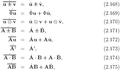
By applying the rules of differentiation, we obtain the identities:
Since, AA-1 = 1,  = 0. Hence, we compute:
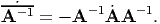 | (2.176) |
A tensor function is a function whose arguments are one or more tensor variables and whose values are scalars, vectors or tensors. The functions Φ(B), u(B), and A(B) are examples of so-called scalar-valued, vector-valued and second order tensor-valued functions of one second order tensor variable B, respectively. In an analogous manner, Φ(v), u(v), and A(v) are scalar-valued, vector-valued and second order tensor-valued functions of one vector variable v, respectively.
Let 𝔇 denote the region of the vector space that is of interest. Then a scalar field Φ, defined on a domain 𝔇, is said to be continuous if
 | (2.177) |
where 𝔙 denote the set of all vectors in the vector space. The properties of continuity are attributed to a vector field u and a tensor field A defined on 𝔇, if they apply to the scalar field u ⋅ a and a ⋅ Ab ∀ a and b ∈𝔙.
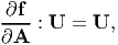
Consider a scalar valued function of one second order tensor variable
A, Φ(A). Assuming the function Φ is continuous in A, the derivative
of Φ with respect to A, denoted by  , is the second order tensor that
satisfies
, is the second order tensor that
satisfies
![∂ Φ d ( ∂ Φ )t ∂ Φ
----⋅ U = ---[Φ(A + sU )]|s=0 = tr( ---- U ) = tr(----Ut),
∂A ds ∂A ∂A](main199x.png) | (2.178) |
for any second order tensor U.
Example: If Φ(A) = det(A), find  both when A is invertible and when it
is not.
both when A is invertible and when it
is not.
Taking trace of the Cayley-Hamilton equation (2.142) and rearranging we get
![1- 3 2 3
det(A ) = 6 [2tr(A ) - 3tr (A )tr(A ) + (tr(A )) ].](main201x.png) | (2.179) |
Hence,
![3 2
∂[det(A-)]= 1[2∂-[tr(A--)]+3 ∂[tr(A-)][(tr(A ))2- tr(A2)]- 3tr(A )∂[tr(A--)]].
∂A 6 ∂A ∂A ∂A](main202x.png) | (2.180) |
Using the properties of trace and dot product we find that
from which, we deduce that using equation (2.178). Substituting equations (2.184) through (2.186) in (2.180) we get
![∂ [det(A )]
----------= (At)2 + I21 - I1At.
∂A](main205x.png) | (2.187) |
If A is invertible, then multiplying (2.142) by A-t and rearranging we get
 | (2.188) |
In light of the above equation, (2.187) reduces to
![∂-[det(A-)] - t
∂A = det(A )A .](main207x.png) | (2.189) |
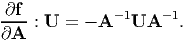
Next, we consider a smooth tensor valued function of one second order tensor
variable A, f(A). As before, the derivative of f with respect to A, denoted by  ,
is the fourth order tensor that satisfies
,
is the fourth order tensor that satisfies
![-∂f-: U = d--[f(A + sU )]|s=0,
∂A ds](main209x.png) | (2.190) |
for any second order tensor U.
It is straight forward to see that when f(A) = A, where A is any second order tensor, then (2.190) reduces to
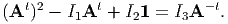
 | (2.191) |
hence,  = I, the fourth order unit tensor where we have used equation
(2.128a).
= I, the fourth order unit tensor where we have used equation
(2.128a).
If f(A) = At where A is any second order tensor, then using (2.190) it can be
shown that  = obtained using equation (2.128b).
Now, say the tensor valued function f is defined only for symmetric tensors,
and that f(S) = S, where S is a symmetric second order tensor. Compute the
derivative of f with respect to S, i.e.,  .
.
First, since the function f is defined only for symmetric tensors, we have to
generalize the function for any tensor. This is required because U is any second
order tensor. Hence, f(S) = f( [A + At]) = (A), where A is any second order
tensor. Now, find the derivative of with respect to A and then rewrite the result
in terms of S. The resulting expression is the derivative of f with respect to S.
Hence,
[A + At]) = (A), where A is any second order
tensor. Now, find the derivative of with respect to A and then rewrite the result
in terms of S. The resulting expression is the derivative of f with respect to S.
Hence,
![1
¯f(A + sU ) = --[A + At + s[U + Ut ]].
2](main215x.png) | (2.192) |
Substituting the above in equation (2.190) we get
![∂¯f-- 1- t
∂A : U = 2[U + U ].](main216x.png) | (2.193) |
Thus,
![∂ ¯f 1
----= -[I + ¯I].
∂A 2](main217x.png) | (2.194) |
Consequently,
![¯
∂f-= ∂-f-= 1[I + ¯I].
∂S ∂A 2](main218x.png) | (2.195) |
Example - 1: Assume that A is an invertible tensor and f(A) = A-1. Then show that
 | (2.196) |
Recalling that all invertible tensors satisfy the relation AA-1 = 1, we obtain
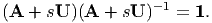 | (2.197) |
Differentiating the above equation with respect to s
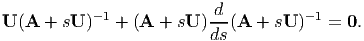 | (2.198) |
Evaluating the above equation at s = 0, and rearranging
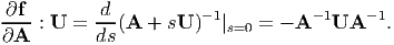 | (2.199) |
Hence proved.
Example - 2: Assume that S is an invertible symmetrical tensor and f(S) =
S-1. Find  .
.
As before generalizing the given function, we have (A) = { [A + At]}-1.
Following the same steps as in the previous example we obtain:
[A + At]}-1.
Following the same steps as in the previous example we obtain:
![[A + At + s(U + Ut )][A + At + s(U + Ut)]-1 = 1.](main225x.png) | (2.200) |
Differentiating the above equation with respect to s and evaluating at s = 0 and rearranging we get
![∂¯f d t t -1 t -1 t t- 1
----: U = 2 --[A + A + s(U + U )] |s=0 = 2 [A + A ] [U + U ][A + A ] .
∂A ds](main226x.png) | (2.201) |
Therefore,
![∂f 1
--- : U = - --S-1[U + Ut ]S-1.
∂S 2](main227x.png) | (2.202) |
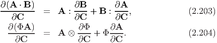
Let Φ be a smooth scalar-valued function and A, B smooth tensor-valued functions of a tensor variable C. Then, it can be shown that
In this section, we consider scalar and vector-valued functions that assign
a scalar and vector to each element in the subset of the set of position
vectors for the points in 3D space. If x denotes the position vector of
points in the 3D space, then  (x) is a function that assigns a scalar Φ to
each point in the 3D space of interest and Φ is called the scalar field. A
few examples of scalar fields are temperature, density, energy. Similarly,
the vector field
(x) is a function that assigns a scalar Φ to
each point in the 3D space of interest and Φ is called the scalar field. A
few examples of scalar fields are temperature, density, energy. Similarly,
the vector field  (x) assigns a vector to each point in the 3D space of
interest. Displacement, velocity, acceleration are a few examples of vector
fields.
(x) assigns a vector to each point in the 3D space of
interest. Displacement, velocity, acceleration are a few examples of vector
fields.
Let 𝔇 denote the region of the 3D space that is of interest, that is the set of position vectors of points that is of interest in the 3D space. Then a scalar field Φ, defined on a domain 𝔇, is said to be continuous if
 | (2.205) |
where 𝔈 denote the set of all position vectors of points in the 3D space and a is a constant vector. The scalar field Φ is said to be differentiable if there exist a vector field w such that
![lim |w (x ) ⋅ a - α -1[Φ (x + αa ) - Φ (x)]| = 0, ∀x ∈ 𝔇, a ∈ 𝔈.
α→0](main232x.png) | (2.206) |
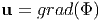
It can be shown that there is at most one vector field, w satisfying the above equation (proof omitted). This unique vector field w is called the gradient of Φ and denoted by grad(Φ).
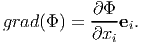
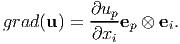
The properties of continuity and differentiability are attributed to a vector field u and a tensor field T defined on 𝔇, if they apply to the scalar field u ⋅ a and a ⋅ Tb ∀ a and b ∈𝔈. Given that the vector field u, is differentiable, the gradient of u denoted by grad(u), is the tensor field defined by
 | (2.207) |
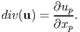
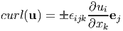
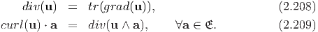
The divergence and the curl of a vector u denoted as div(u) and curl(u), are respectively scalar valued and vector valued and are defined by
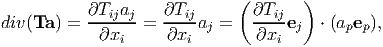
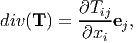
When the tensor field T is differentiable, its divergence denoted by div(T), is the vector field defined by
 | (2.210) |
If grad(Φ) exist and is continuous, Φ is said to be continuously differentiable and this property extends to u and T if grad(u⋅a) and grad(a⋅Tb) exist and are continuous for all a, b ∈𝔈.
An important identity: For a continuously differentiable vector field, u
 | (2.211) |
(Proof omitted)
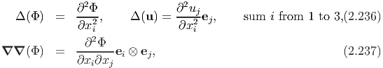
Let Φ and u be some scalar and vector field respectively. Then, the Laplacian operator, denoted by Δ (or by ∇2), is defined as
 | (2.212) |
The Hessian operator, denoted by ∇∇ is defined as
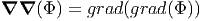 | (2.213) |
If a vector field u is divergence free (i.e. div(u) = 0) then it is called solenoidal. It is called irrotational if curl(u) = o. It can be established that
 | (2.214) |
Consequently, if a vector field, u is both solenoidal and irrotational, then Δ(u) = o (follows from the above equation) and such a vector field is said to be harmonic. If a scalar field Φ satisfies Δ(Φ) = 0, then Φ is said to be harmonic.
Potential theorem: Let u be a smooth point field on an open or closed
simply connected region  and let curl(u) = o. Then there is a continuously
differentiable scalar field on such that
and let curl(u) = o. Then there is a continuously
differentiable scalar field on such that
 | (2.215) |
From the definition of grad (2.207), it can be seen that it is a linear operator. That is,
 | (2.216) |
Consequently, all other operators div, Δ are also linear operators.
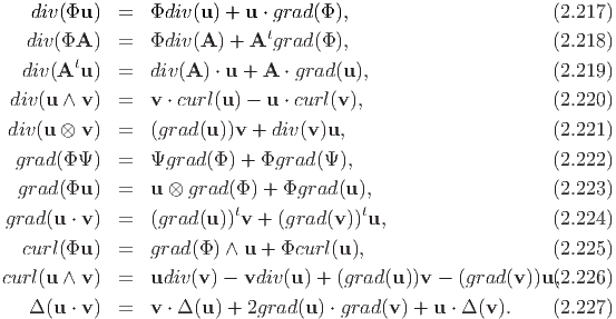
Before concluding this section we collect a few identities that are useful subsequently. Here Φ, Ψ are scalar fields, u, v are vector fields and A is second order tensor field.
Till now, in this section we defined all the quantities in closed form but we require them in component form to perform the actual calculations. This would be the focus in the reminder of this section. In the following, let ei denote the Cartesian basis vectors and xi i = 1, 2, 3, the Cartesian coordinates.
Let Φ be differentiable scalar field, then it follows from equation (2.206), on
replacing a by the base vectors ei in turn, that the partial derivatives  exist in
𝔇 and that, moreover, wi =
exist in
𝔇 and that, moreover, wi =  . Hence
 | (2.228) |
Let u be differentiable vector field in 𝔇 and a some constant vector in 𝔈. Then, using (2.228) we compute
 | (2.229) |
where ap and up are the Cartesian components of a and u respectively. Consequently, appealing to definition (2.207) we obtain
 | (2.230) |
Then, according to the definition for divergence, (2.208)
 | (2.231) |
Next, we compute div(u ∧ a) to be
 | (2.232) |
using (2.231). Comparing the above result with the definition of curl in (2.209) we infer
 | (2.233) |
Finally, let T be a differentiable tensor field in 𝔇, then we compute
 | (2.234) |
using equation (2.231). Then, we infer
 | (2.235) |
from the definition (2.210).
The component form for the other operators, namely Laplacian and Hessian can be obtained as
Above we obtained the components of the different operators in Cartesian coordinate system, we shall now proceed to obtain the same with respect to other coordinate systems. While using the method illustrated here we could obtain the components in any orthogonal curvilinear system, we choose the cylindrical polar coordinate system for illustration.
First, we outline a general procedure to find the basis vectors for a given orthogonal curvilinear coordinates. A differential vector dp in the 3D vector space is written as dp = dxiei relative to Cartesian coordinates. The same coordinate independent vector in orthogonal curvilinear coordinates is written as
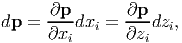 | (2.238) |
where zi denotes curvilinear coordinates. But
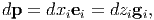 | (2.239) |
where gi is the basis vectors in the orthogonal curvilinear coordinates. Thus,
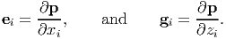 | (2.240) |
Comparing equations (2.239) and (2.240) we obtain the desired transformation relation between the bases to be:
 | (2.241) |
The basis gi so obtained will vary from point to point in the Euclidean space and will be orthogonal (by the choice of curvilinear coordinates) at each point but not orthonormal. Hence we define
 | (2.242) |
and use these as the basis vectors for the orthogonal curvilinear coordinates.
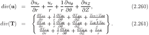
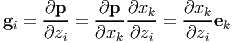
Let (x,y,z) denote the coordinates of a typical point in Cartesian coordinate system and (r,θ,Z) the coordinates of a typical point in cylindrical polar coordinate system. Then, the coordinate transformation from cylindrical polar to Cartesian and vice versa is given by:
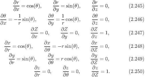
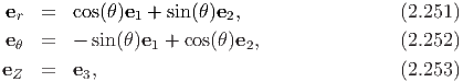
Consequently, the orthonormal cylindrical polar basis vectors (er,eθ,eZ) and Cartesian basis vectors (e1,e2,e3) are related through the equations
Now, we can compute the components of grad(Φ) in cylindrical polar coordinates. Towards this, we obtain
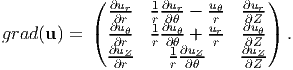
To obtain the components of grad(u) one can follow the same procedure outlined above or can compute the same using the above result and the definition of grad (2.207) as detailed below:
where we have used the following identities: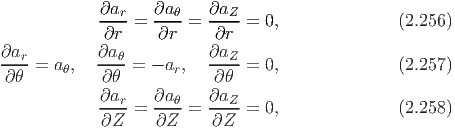
 | (2.259) |
Using the techniques illustrated above the following identities can be established:
Suppose u(x) is a vector field defined on some convex three dimensional region,
in physical space with volume v and on a closed surface a bounding this
volume2
and u(x) is continuous in and continuously differentiable in the interior of .
Then,
 | (2.262) |
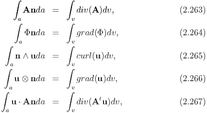
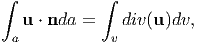
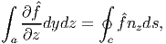
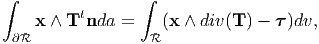
where, n is the outward unit normal field acting along the surface a, dv and da are infinitesimal volume and surface element, respectively. Proof of this theorem is beyond the scope of these notes.
Using (2.262) the following identities can be established:
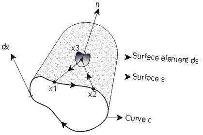
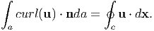
where Φ, u, A are continuously differentiable scalar, vector and tensor fields defined in v and continuous in v and n is the outward unit normal field acting along the surface a.Stokes theorem relates a surface integral, which is valid over any open surface a, to a line integral around the bounding single simple closed curve c in three dimensional space. Let dx denote the tangent vector to the curve, c and n denote the outward unit vector field n normal to s. The curve c has positive orientation relative to n in the sense shown in figure 2.3. The indicated circuit with the adjacent points 1, 2, 3 (1, 2 on curve c and 3 an interior point of the surface s) induced by the orientation of c is related to the direction of n (i.e., a unit vector normal to s at point 3) by right-hand screw rule. For a continuously differentiable vector field u defined on some region containing a, we have
 | (2.268) |
Let Φ and u be continuously differentiable scalar and vector fields defined on a and c and n is the outward drawn normal to a. Then, the following can be shown:
![∮ ∫
Φdx = n ∧ grad(Φ )da, (2.269)
∮ c ∫a
t
u ∧ dx = [div(u)n - (grad (u))n ]da. (2.270)
c a](main270x.png)
Finally, we record Greens’s theorem. We do this first for simply connected domain and then for multiply connected domain. If any curve within the domain can be shrunk to a point in the domain without leaving the domain, then such a domain is said to be simply connected. A domain that is not simply connected is said to be multiply connected.
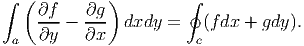
Applying Stoke’s theorem, (2.268) to a planar simply connected domain with the vector field given as u = f(x,y)e1 + g(x,y)e2,
 | (2.271) |
The above equation (2.271) when f(x,y) = 0 reduces to
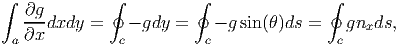 | (2.272) |
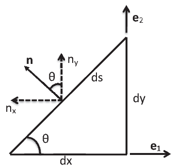
where θ is the angle made by the tangent to the curve c with e1 and nx is the component of the unit normal n along e1 direction, refer to figure 2.4. Then, when g(x,y) = 0 equation (2.271) yields,
 | (2.273) |
where ny is the component of the unit normal along the e2 direction.
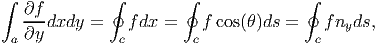
Similarly, applying Stoke’s theorem (2.268) to a vector field, u =  (y,z)e2 +
ĝ(y,z)e3 defined over a planar simply connected domain,
(y,z)e2 +
ĝ(y,z)e3 defined over a planar simply connected domain,
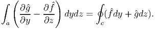 | (2.274) |
The above equation (2.274) when  (y,z) = 0 reduces to
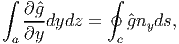 | (2.275) |
where ny is the component of the normal to the curve along the e2 direction and when ĝ(y,z) = 0 yields
 | (2.276) |
where nz is the component of the normal to the curve along the e3 direction.
In a simply connected domain, the region of interest has a single simple closed curve. In a multiply connected domain, the region of interest has several simple closed curves, like the one shown in figure 2.5. If the line integrals are computed by traversing in the direction shown in figure 2.5,
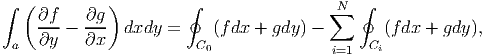 | (2.277) |
where the functions f and g are continuously differentiable in the domain, C0 is the outer boundary of the domain, Ci’s are the boundary of the voids in the interior of the domain and we have assumed that there are N such voids in the domain. We emphasize again our assumption that we transverse the interior voids in the same sense as the outer boundary.
The above equation (2.277) when f(x,y) = 0 reduces to
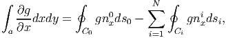 | (2.278) |
where nxi is the component of the unit normal n along e 1 direction of the ith curve. Then, when g(x,y) = 0 equation (2.277) yields,
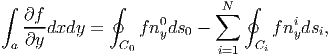 | (2.279) |
where nyi is the component of the unit normal along the e 2 direction of the ith curve.
In this chapter, we looked at the mathematical tools required to embark on a study of mechanics. In particular, we began with a study on algebra of tensors and then graduated to study tensor calculus. Most of the mathematical results that we would be using is summarized in this chapter.
![I3 = {[tr(A )]3 - 3tr(A )tr(A2 ) + 2tr(A3 )}∕6](main285x.png) |
for an arbitrary tensor A.
 exists, prove that
 |
 =
I3A-1
=
I3A-1
 =
=  div(u) -
 u ⋅ grad(ϕ)
 |
For this tensor find the following:
 i} of basis vectors with transformation law
  2 = - sin(θ)e1 + cos(θ)e2,
 3 = e3. The origin of the new coordinate system coincides with the old
origin.
3 = e3. The origin of the new coordinate system coincides with the old
origin.
 1 in terms of the old set {ei} of basis vectors
 i} of basis vectors
 i} basis and establish the relationship between the
components of r represented using {ei} basis and {
i} basis and establish the relationship between the
components of r represented using {ei} basis and { i} basis.
 |
relative to a Cartesian orthonormal basis, {ei}, determine
 i} with respect to the
basis, {ei}, so that the stress tensor has a matrix representation
of the form, T = diag[p1,p2,p3] when expressed with respect to
the {
i} with respect to the
basis, {ei}, so that the stress tensor has a matrix representation
of the form, T = diag[p1,p2,p3] when expressed with respect to
the { i} basis
 i}.
i}.
 i}
when
i}
when  1 = (
1 = ( e1 + e2)∕2,
  2 = (-e1 +
  e2)∕2,
  3 = e3. be a regular region and T a tensor field which is continuous in and
continuously differentiable in the interior of . Show that,
3 = e3. be a regular region and T a tensor field which is continuous in and
continuously differentiable in the interior of . Show that,
 |
where x is the position of a representative point of and τ is the axial
vector of T - Tt. (Hint: Make use of the identity obtained in problem
23.)
![div(T ) =
( ∂T )
|{ ∂T∂rrr-+ 1r ∂T∂θrθ-+ rco1s(θ)-∂ϕϕr+ 1r[2Trr - T θθ - Tϕϕ] |}
∂Trθ-+ 1∂Tθθ-+ ---1--∂Tϕθ+ 1[2T + T + (T - T )tan (θ )] ,
|( ∂T∂r r∂∂Tθ rcos(θ)∂∂Tϕ r rθ θr θθ ϕϕ |)
∂rrϕ-+ 1r ∂θθϕ-+ rco1s(θ)-∂ϕϕϕ+ 1r[2Trϕ + Tϕr + (T ϕθ + T θϕ) tan(θ)]](main314x.png) |
![tr(A + sU ) = tr(A) + s1 ⋅ U, (2.181)
tr([A + sU ]2) = tr(A2) + 2sAt ⋅ U + s2tr(U2 ), (2.182)
3 3 t 2 2 t 2 3 3
tr([A + sU ]) = tr(A ) + 3s(A ) ⋅ U + 3s A ⋅ U + s tr(U )(,2.183)](main203x.png)
![∂[tr(A )]
--------- = 1, (2.184)
∂A 2
∂[tr(A--)]- = 2At, (2.185)
∂A
∂[tr(A3 )] t2
---------- = 3(A ) , (2.186)
∂A](main204x.png)
![( ∂ 1 ∂ ∂ )
grad (u ⋅ a) = ---er + ----e θ +---ez (urar + uθaθ + uZ aZ)
[∂r r ∂θ ∂z ]
∂ur ∂uθ ∂uZ
= ----ar + ---a θ +---- aZ er
∂r [ ∂r ∂r ]
1- ∂ur- ∂uθ- ∂uZ-
+ r ∂ θ ar + ura θ + ∂θ a θ - uθar + ∂θ aZ eθ
[ ]
+ ∂urar + ∂u-θaθ + ∂uZ-aZ eZ , (2.255)
∂Z ∂Z ∂Z](main263x.png)