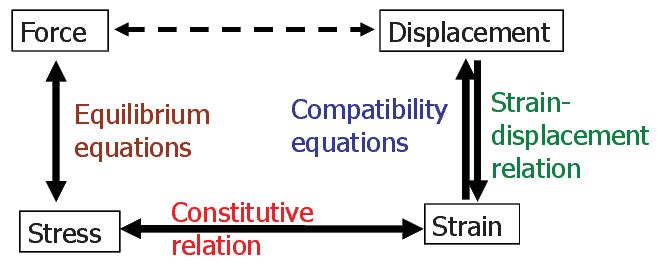
Figure 1.1: Basic concepts and equations in mechanics
In this course too we shall be studying the same four concepts and four equations. While in the “mechanics of materials” course, one was introduced to the various components of the stress and strain, namely the normal and shear, in the problems that was solved not more than one component of the stress or strain occurred simultaneously. Here we shall be studying these problems in which more than one component of the stress or strain occurs simultaneously. Thus, in this course we shall be generalizing these concepts and equations to facilitate three dimensional analysis of structures.
Before venturing into the generalization of these concepts and equations, a few drawbacks of the definitions and ideas that one might have acquired from the previous course needs to be highlighted and clarified. This we shall do in sections 1.1 and 1.2. Specifically, in section 1.1 we look at the four concepts in mechanics and in section 1.2 we look at the equations in mechanics. These sections also serve as a motivation for the mathematical tools that we would be developing in chapter 2. Then, in section 1.3 we look into various idealizations of the response of materials and the mathematical framework used to study them. However, in this course we shall be only focusing on the elastic response or more precisely, non-dissipative response of the materials. Finally, in section 1.4 we outline three ways by which we can solve problems in mechanics.
Force is a mathematical idea to study the motion of bodies. It is not “real” as many think it to be. However, it can be associated with the twitching of the muscle, feeling of the burden of mass, linear translation of the motor, so on and so forth. Despite seeing only displacements we relate it to its cause the force, as the concept of force has now been ingrained.
Let us see why force is an idea that arises from mathematical need. Say, the position1 (xo) and velocity (vo) of the body is known at some time, t = to, then one is interested in knowing where this body would be at a later time, t = t1. It turns out that mathematically, if the acceleration (a) of the body at any later instant in time is specified then the position of the body can be determined through Taylor’s series. That is if
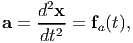 | (1.1) |
then from Taylor’s series
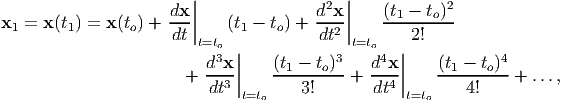 | (1.2) |
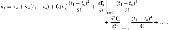 | (1.3) |
It is pertinent to point out that this function fa could also be prescribed using the position, x and velocity, v of the body which are themselves function of time, t and hence fa would still be a function of time. Thus, fa = g(x(t),v(t),t). However, fa could not arbitrarily depend on t, x and v. At this point it suffices to say that the other two laws of Newton and certain objectivity requirements have to be met by this function. We shall see what these objectivity requirements are and how to prescribe functions that meet this requirement subsequently in chapter - 6.
Next, let us understand what kind of quantity is force. In other words is force a scalar or vector and why? Since, position is a vector and acceleration is second time derivative of position, it is also a vector. Then, it follows from equation (1.1) that fa also has to be a vector. Therefore, force is a vector quantity. Numerous experiments also show that addition of forces follow vector addition law (or the parallelogram law of addition). In chapter 2 we shall see how the vector addition differs from scalar addition. In fact it is this addition rule that distinguishes a vector from a scalar and hence confirms that force is a vector.
As a summary, we showed that force is a mathematical construct which is used to mathematically describe the motion of bodies.
As is evident from figure 1.1, stress is a quantity derived from force. The commonly stated definitions in an introductory course in mechanics for stress are:
While the first definition tells how to compute the stress from the force, this definition holds only for simple loading case. One can construct a number of examples where definition 1 does not hold. The following two cases are presented just as an example. Case -1: A cantilever beam of rectangular cross section with a uniform pressure, p, applied on the top surface, as shown in figure 1.2a. According to the definition 1 the stress in the beam should be p, but it is not. Case -2: An annular cylinder subjected to a pressure, p at its inner surface, as shown in figure 1.2b. The net force acting on the cylinder is zero but the stresses are not zero at any location. Also, the stress is not p, anywhere in the interior of the cylinder. This being the state of the first definition, the second definition is of little use as it does not tell how to compute the stress. These definitions does not tell that there are various components of the stress nor whether the area over which the force is considered to be distributed is the deformed or the undeformed. They do not distinguish between traction (or stress vector), t(n) and stress tensor, σ.
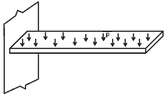 (a) A cantilever beam with uniform
pressure applied on its top surface.
(a) A cantilever beam with uniform
pressure applied on its top surface. 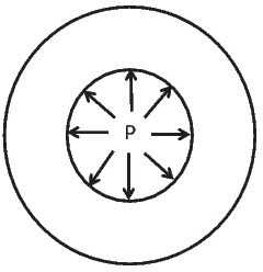 (b) An annular cylinder subjected to
internal pressure.
(b) An annular cylinder subjected to
internal pressure.
Traction is the distributed force acting per unit area of a cut surface or boundary of the body. This traction apart from varying spatially and temporally also depends on the plane of cut characterized by its normal. This quantity integrated over the cut surface gives the net force acting on that surface. Consequently, since force is a vector quantity this traction is also a vector quantity. The component of the traction along the normal direction4 , n is called as the normal stress (σ(n)). The magnitude of the component of the traction5 acting parallel to the plane is called as the shear stress (τ(n)).
If the force is distributed over the deformed area then the corresponding traction is called as the Cauchy traction (t(n)) and if the force is distributed over the undeformed or original area that traction is called as the Piola traction (p(n)). If the deformed area does not change significantly from the original area, then both these traction would have nearly the same magnitude and direction. More details about these traction is presented in chapter 4.
The stress tensor, is a linear function (crudely, a matrix) that relates the normal vector, n to the traction acting on that plane whose normal is n. The stress tensor could vary spatially and temporally but does not change with the plane of cut. Just like there is Cauchy and Piola traction, depending on over which area the force is distributed, there are two stress tensors. The Cauchy (or true) stress tensor, σ and the Piola-Kirchhoff stress tensor (P). While these two tensors may nearly be the same when the deformed area is not significantly different from the original area, qualitatively these tensors are different. To satisfy the moment equilibrium in the absence of body couples, Cauchy stress tensor has to be symmetric tensor (crudely, symmetric matrix) and Piola-Kirchhoff stress tensor cannot be symmetric. In fact the transpose of the Piola-Kirchhoff stress tensor is called as the engineering stress or nominal stress. Moreover, there are many other stress measures obtained from the Cauchy stress and the gradient of the displacement which shall be studied in chapter 4.
The difference between the position vectors of a material particle at two different instances of time is called as displacement. In general, the displacement of the material particle would depend on time; the instances between which the displacement is sought. It is also possible that different particles get displaced differently between the same two instances of time. Thus, displacement in general varies spatially and temporally. Displacement is what can be observed and measured. Forces, traction and stress tensors are introduced to explain (or mathematically capture) this displacement.
The displacement field is at least differentiable twice temporally so that acceleration could be computed. This stems from the observations that the location or velocity of the body does not change abruptly. Similarly, the basic tenant of continuum mechanics is that the displacement field is continuous spatially and is piecewise differentiable spatially at least twice. That is while the displacement field is required to be continuous over the entire body it is required to be twice differentiable not necessarily over the entire body but only on subsets of the body. Thus, in continuum mechanics interpenetration of two surfaces or separation and formation of new surfaces is precluded. The validity of the theory stops just before the body fractures. Notwithstanding this many attempt to use continuum mechanics concepts to understand the process of fracture.
A body is said to undergo rigid body displacement if the distance between any two particles that belongs to the body remains unchanged. That is in a rigid body displacement the particles that belong to a body do not move relative to each other. A body is said to be rigid if it always undergoes only rigid body displacement under action of any force. On the other hand, a body is said to be deformable if it allows relative displacement of its particles under the action of some force. Though, all real bodies are deformable, at times one could idealize a given body as rigid under the action of certain forces.
One observes that rigid body displacements of the body does not give raise to any stresses. Further, stresses are induced only when there is relative displacement of the material particles. Consequently, one requires a measure (or metric) for this relative displacement so that it can be related to the stress. The unique measure of relative displacement is the stretch ratio, λ(A), defined as the ratio of the deformed length to the original length of a material fiber along a given direction, A. (Note that here A is a unit vector.) However, this measure has the drawback that when the body is not deformed the stretch ratio is 1 (by virtue of the deformed length being same as the original length) and hence inconvenient to write the constitutive relation of the form
 | (1.4) |
where σ(A) denotes the normal stress on a plane whose normal is A. Since the stress is zero when the body is not deformed, the function f should be such that f(1) = 0. Mathematical implementation of this condition that f(1) = 0 and that f be a one to one function is thought to be difficult when f is a nonlinear function of λ(A). Consequently, another measure of relative displacement is sought which would be 0 when the body is not deformed and less than zero when compressed and greater than zero when stretched. This measure is called as the strain, ϵ(A). There is no unique way of obtaining the strain from the stretch ratio. The following functions satisfy the requirement of the strain:
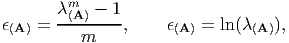 | (1.5) |
where m is some real number and ln stands for natural logarithm. Thus, if m = 1 in (1.5a) then the resulting strain is called as the engineering strain, if m = -1, it is called as the true strain, if m = 2 it is Cauchy-Green strain. The second function wherein ϵ(A) = ln(λ(A)), is called as the Hencky strain or the logarithmic strain.
Just like the traction and hence the normal stress changes with the orientation of the plane, the stretch ratio also changes with the orientation along which it is measured. We shall see in chapter 3 that a tensor called the Cauchy-Green deformation tensor carries all the information required to compute the stretch ratio along any direction. This is akin to the stress tensor which when known we could compute the traction or the normal stress in any plane.
Having gained a superficial understanding of the four concepts in mechanics namely the force, stress, displacement and strain, let us look at the four equations that connect these concepts and the reasoning used to obtain them.
Equilibrium equations are Newton’s second law which states that the rate of change of linear momentum would be equal in magnitude and direction to the net applied force. Deformable bodies are subjected to two kinds of forces, namely, contact force and body force. As the name suggest the contact force arises by virtue of the body being in contact with its surroundings. Traction arises only due to these contact force and hence so does the stress tensor. The magnitude of the contact force depends on the contact area between the body and its surroundings. On the other hand, the body forces are action at a distance forces. Examples of body force are gravitational force, electromagnetic force. The magnitude of these body forces depend on the mass of the body and hence are generally expressed as per unit mass of the body and denoted by b.
On further assuming that the Newton’s second law holds for any subpart of the body and that the stress field is continuously differentiable within the body the equilibrium equations can be written as:
 | (1.6) |
where ρ is the density, a is the acceleration and the mass is assumed to be conserved. Detail derivation of the above equation is given in chapter 5. The meaning of the operator div(⋅) can be found in chapter 2.
Also, the rate of change of angular momentum must be equal to the net applied moment on the body. Assuming that the moment is generated only by the contact forces and body forces, this condition requires that the Cauchy stress tensor to be symmetric. That is in the absence of body couples, σ = σt, where the superscript (⋅)t denotes the transpose. Here again the assumptions made to obtain the force equilibrium equation (1.6) should hold. See chapter 5 for detailed derivation.
The relationship that connects the displacement field with the strain is called as the strain displacement relationship. As pointed out before there is no unique definition of the strain and hence there are various strain tensors. However, all these strains are some function of the gradient of the deformation field, F; commonly called as the deformation gradient. The deformation field is a function that gives the position vector of any material particle that belongs to the body at any instance in time with the material particle identified by its location at some time to. Then, in chapter 3 we show that, the stretch ratio along a given direction A is,
 | (1.7) |
where C = FtF, is called as the right Cauchy-Green deformation tensor. When the body is undeformed, F = 1 and hence, C = 1 and λ(A) = 1. Instead of looking at the deformation field, one can develop the expression for the stretch ratio, looking at the displacement field too. Now, the displacement field can be a function of the coordinates of the material particles in the reference or undeformed state or the coordinates in the current or deformed state. If the displacement is a function of the coordinates of the material particles in the reference configuration it is called as Lagrangian representation of the displacement field and the gradient of this Lagrangian displacement field is called as the Lagrangian displacement gradient and is denoted by H. On the other hand if the displacement is a function of the coordinates of the material particle in the deformed state, such a representation of the displacement field is said to be Eulerian and the gradient of this Eulerian displacement field is called as the Eulerian displacement gradient and is denoted by h. Then it can be shown that (see chapter 3),
 | (1.8) |
where, 1 stands for identity tensor (see chapter 2 for its definition). Now, the right Cauchy-Green deformation tensor can be written in terms of the Lagrangian displacement gradient as,
 | (1.9) |
Note that the if the body is undeformed then H = 0. Hence, if one cannot see the displacement of the body then it is likely that the components of the Lagrangian displacement gradient are going to be small, say of order 10-3. Then, the components of the tensor HtH are going to be of the order 10-6. Hence, the equation (1.9) for this case when the components of the Lagrangian displacement gradient is small can be approximately calculated as,
 | (1.10) |
where
![[ ]
ϵL = 1-H + Ht ,
2](main14x.png) | (1.11) |
is called as the linearized Lagrangian strain. We shall see in chapter 3 that when the components of the Lagrangian displacement gradient is small, the stretch ratio (1.7) reduces to
 | (1.12) |
Thus we find that ϵL contains information about changes in length along any given direction, A when the components of the Lagrangian displacement gradient are small. Hence, it is called as the linearized Lagrangian strain. We shall in chapter 3 derive the various strain tensors corresponding to the various definition of strains given in equation (1.5).
Further, since FF-1 = 1, it follows from (1.8) that
 | (1.13) |
which when the components of both the Lagrangian and Eulerian displacement gradient are small can be approximated as H = h. Thus, when the components of the Lagrangian and Eulerian displacement gradients are small these displacement gradients are the same. Hence, the Eulerian linearized strain defined as,
![1-[ t]
ϵE = 2 h + h ,](main17x.png) | (1.14) |
and the Lagrangian linearized strain, ϵL would be the same when the components of the displacement gradients are small.
Equation (1.14) is the strain displacement relationship that we would use to solve boundary value problems in this course, as we limit ourselves to cases where the components of the Lagrangian and Eulerian displacement gradient is small.
It is evident from the definition of the linearized Lagrangian strain, (1.11) that it is a symmetric tensor. Hence, it has only 6 independent components. Now, one cannot prescribe arbitrarily these six components since a smooth differentiable displacement field should be obtainable from this six prescribed components. The restrictions placed on how this six components of the strain could vary spatially so that a smooth differentiable displacement field is obtainable is called as compatibility equation. Thus, the compatibility condition is
 | (1.15) |
The derivation of this equation as well as the components of the curl(⋅) operator in Cartesian coordinates is presented in chapter 3.
It should also be mentioned that the compatibility condition in case of large deformations is yet to be obtained. That is if the components of the right Cauchy-Green deformation tensor, C is prescribed, the restrictions that have to be placed on these prescribed components so that a smooth differentiable deformation field could be obtained is unknown, except for some special cases.
Broadly constitutive relation is the equation that relates the stress (and stress rates) with the displacement gradient (and rate of displacement gradient). While the above three equations - Equilibrium equations, strain-displacement relation, compatibility equations - are independent of the material that the body is made up of and/or the process that the body is subjected to, the constitutive relation is dependent on the material and the process. Constitutive relation is required to bring in the dependance of the material in the response of the body and to have as many equations as there are unknowns, as will be shown in chapter 6.
The fidelity of the predictions, namely the likely displacement or stress for a given force depends only on the constitutive relation. This is so because the other three equations are the same irrespective of the material that the body is made up of. Consequently, a lot of research is being undertaken to arrive at better constitutive relations for materials.
It is difficult to have a constitutive relation that could describe the response of a material subjected to any process. Hence, usually constitutive relations are prescribed for a particular process that the material undergoes. The variables in the constitutive relation depends on the process that is being studied. The same material could undergo different processes depending on the stimuli; for example, the same material could respond elastically or plastically depending on say, the magnitude of the load or temperature. Hence it is only apt to qualify the process and not the material. However, it is customary to qualify the material instead of the process too. This we shall desist.
Traditionally, the constitutive relation is said to depend on whether the given material behaves like a solid or fluid and one elaborates on how to classify a given material as a solid or a fluid. A material that is not a solid is defined as a fluid. This means one has to define what a solid is. A couple of definitions of a solid are listed below:
Though these definitions are intuitive they are ambiguous. A class of materials called “viscoelastic solids”, neither take the shape of the container nor resist shear forces without continuously deforming. Also, the same material would behave like a solid, like a mixture of a solid and a fluid or like a fluid depending on say, the temperature and the mechanical stress it is being subjected to. These prompts us to say that a given material behaves in a solid-like or fluid-like manner. However, as we shall see, this classification of a given material as solid or fluid is immaterial. If one appeals to thermodynamics for the classification of the processes, the response of materials could be classified based on (1) Whether there is conversion of energy from one form to another during the process, and (2) Whether the process is thermodynamically equilibrated. Though, in the following section, we classify the response of materials based on thermodynamics, we also give the commonly stated definitions and discuss their shortcomings. In this course, as well as in all these classifications, it is assumed that there are no chemical changes occurring in the body and hence the composition of the body remains a constant.
First, it should be clarified that one should not get confused with the real body and its mathematical idealization. Modeling is all about idealizations that lead to predictions that are close to observations. To illustrate, the earth and the sun are assumed as point masses when one is interested in planetary motion. The same earth is assumed as a rigid sphere if one is interested in studying the eclipse. These assumptions are made to make the resulting problem tractable without losing on the required accuracy. In the same sprit, the all material responses, some amount of mechanical energy is converted into other forms of energy. However, in some cases, this loss in the mechanical energy is small that it can be idealized as having no loss, i.e., a non-dissipative process.
A response is said to be non-dissipative if there is no conversion of mechanical energy to other forms of energy, namely heat energy. Commonly, a material responding in this fashion is said to be elastic. The common definitions of elastic response,
The first definition is of little use, because it requires one to do a complimentary process (unloading) to decide on whether the process that needs to be classified as being elastic. The second definition, though useful for deciding on the variables in the constitutive relation, it also requires one to do a complimentary process (unload and load again) to decide on whether the first process is elastic. The definition based on thermodynamics does not suffer from this drawback. In chapter 6 we provide examples where these three definitions are not equivalent. However, many processes (approximately) satisfy all the three definitions.
This class of processes also proceeds through thermodynamically equilibrated states. That is, if the body is isolated at any instant of loading (or displacement) then the stress, displacement, internal energy, entropy do not change with time.
Ideal gas, a fluid is the best example of a material that responds in a non-dissipative manner. Metals up to a certain stress level, called the yield stress, are also idealized as responding in a non dissipative manner. Thus, the notion that only solids respond in a non-dissipative manner is not correct.
Thus, for these non-dissipative, thermodynamically equilibrated processes the
Cauchy stress and the deformation gradient can in general be related through
an implicit function. That is, for isotropic materials (see chapter 6 for
when a material is said to be isotropic), f(σ,F) = 0. However, in classical
elasticity it is customary to assume that Cauchy stress in a isotropic material
is a function of the deformation gradient, σ =  (F). On requiring the
restriction6
due to objectivity and second law of thermodynamics to hold, it can be shown
that if σ =
(F). On requiring the
restriction6
due to objectivity and second law of thermodynamics to hold, it can be shown
that if σ =  (F), then
![[ ]
σ = ∂ψR-1 + 2-- ∂ψR-B - ∂ψR-B -1 ,
∂J3 J3 ∂J1 ∂J2](main21x.png) | (1.16) |
where ψR =  R(J1,J2,J3) is the Helmoltz free energy defined per unit volume in
the reference configuration, also called as the stored energy, B = FFt and J
1 =
tr(B), J2 = tr(B-1), J
3 =
R(J1,J2,J3) is the Helmoltz free energy defined per unit volume in
the reference configuration, also called as the stored energy, B = FFt and J
1 =
tr(B), J2 = tr(B-1), J
3 =  . When the components of the displacement
gradient is small, then (1.16) reduces to,
. When the components of the displacement
gradient is small, then (1.16) reduces to,
 | (1.17) |
on neglecting the higher powers of the Lagrangian displacement gradient and where λ and μ are called as the Lamè constants. The equation (1.17) is the famous Hooke’s law for isotropic materials. In this course Hooke’s law is the constitutive equation that we shall be using to solve boundary value problems.
Before concluding this section, another misnomer needs to be clarified. As can be seen from equation (1.16) the relationship between Cauchy stress and the displacement gradient can be nonlinear when the response is non-dissipative. Only sometimes as in the case of the material obeying Hooke’s law is this relationship linear. It is also true that if the response is dissipative, the relationship between the stress and the displacement gradient is always nonlinear. However, nonlinear relationship between the stress and the displacement gradient does not mean that the response is dissipative. That is, nonlinear relationship between the stress and the displacement gradient is only a necessary condition for the response to be dissipative but not a sufficient condition.
A response is said to be dissipative if there is conversion of mechanical energy to other forms of energy. A material responding in this fashion is popularly said to be inelastic. There are three types of dissipative response, which we shall see in some detail.
A material is said to deform plastically if the deformation process proceeds through thermodynamically equilibrated states but is dissipative. That is, if the body is isolated at any instant of loading (or displacement) then the stress, displacement, internal energy, entropy do not change with time. By virtue of the process being dissipative, the stress at an instant would depend on the history of the deformation. However, the stress does not depend on the rate of loading or displacement by virtue of the process proceeding through thermodynamically equilibrated states.
For plastic response, the classical constitutive relation is assumed to be of the form,
 | (1.18) |
where Fp, q 1, q2 are internal variables whose values could change with deformation and/or stress. For illustration, we have used two scalar internal variables and one second order tensor internal variable while there can be any number of tensor or scalar internal variables. In some theories the internal variables are given a physical interpretation but in general, these variable need not have any meaning and are proposed for mathematical modeling purpose only.
Thus, when a material deforms plastically, it does not return back to its original shape when unloaded; there would be a permanent deformation. Hence, the process is irreversible. The response does not depend on the rate of loading (or displacement). Metals like steel at room temperature respond plastically when stressed above a particular limit, called the yield stress.
If the dissipative process proceeds through states that are not in thermodynamic equilibrium7 , then it is said to be viscoelastic. Therefore, if a body is isolated at some instant of loading (or displacement) then the displacement (or the stress) continues to change with time. A viscoelastic material when subjected to constant stress would result in a deformation that changes with time which is called as creep. Also, when a viscoelastic material is subjected to a constant deformation field, its stress changes with time and this is called as stress relaxation. This is in contrary to a elastic or plastic material which when subjected to a constant stress would have a constant strain.
The constitutive relation for a viscoelastic response is of the form,
 | (1.19) |
where  denotes the time derivative of stress and
  time derivative of the
deformation gradient. Though here we have truncated to first order time
derivatives, the general theory allows for higher order time derivatives
too.
time derivative of the
deformation gradient. Though here we have truncated to first order time
derivatives, the general theory allows for higher order time derivatives
too.
Thus, the response of a viscoelastic material depends on the rate at which it is loaded (or displaced) apart from the history of the loading (or displacement). The response of a viscoelastic material changes depending on whether load is controlled or displacement is controlled. This process too is irreversible and there would be unrecovered deformation immediately on removal of the load. The magnitude of unrecovered deformation after a long time (asymptotically) would tend to zero or remain the same constant value that it is immediately after the removal of load.
Constitutive relations of the form,
 | (1.20) |
which is a special case of the viscoelastic constitutive relation (1.19), is that of a viscous fluid.
In some treatments of the subject, a viscoelastic material would be said to be a combination of a viscous fluid and an elastic solid and the viscoelastic models are obtained by combining springs and dashpots. There are several philosophical problems associated with this viewpoint about which we cannot elaborate here.
This process too is dissipative and proceeds through states that are not in thermodynamic equilibrium. However, in order to model this class of response the constitutive relation has to be of the form,
 | (1.21) |
where Fp, q 1, q2 are the internal variables whose values could change with deformation and/or stress. Their significance is same as that discussed for plastic response. As can be easily seen the constitutive relation form for the viscoplastic response (1.21) encompasses viscoelastic, plastic and elastic response as a special case.
In this case, constant load causes a deformation that changes with time. Also, a constant deformation causes applied load to change with time. The response of the material depends on the rate of loading or displacement. The process is irreversible and there would be unrecovered deformation on removal of load. The magnitude of this unrecovered deformation varies with rate of loading, time and would tend to a value which is not zero. This dependance of the constant value that the unrecovered deformation tends on the rate of loading, could be taken as the characteristic of viscoplastic response.
Figure 1.3 shows the typical variation in the strain for various responses when the material is loaded, held at a constant load and unloaded, as discussed above. This kind of loading is called as the creep and recovery loading, helps one to distinguish various kinds of responses.
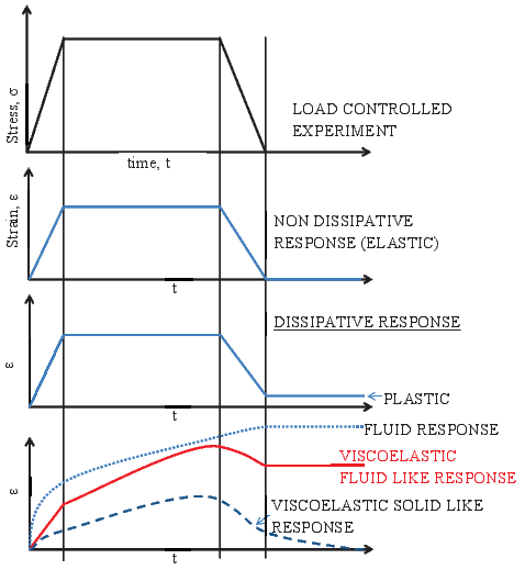
As mentioned already, in this course we shall focus on the elastic or non-dissipative response only.
A boundary value problem is one in which we specify the traction applied on the surface of a body and/or displacement of the boundary of a body and are interested in finding the displacement and/or the stress at any interior point in the body or on part of the boundary where they were not specified. This specification of the boundary traction and/or displacement is called as boundary condition. The boundary condition is in a sense constitutive relation for the boundary. It tells how the body and its surroundings interact. Thus, in a boundary value problem one needs to prescribe the geometry of the body, the constitutive relation for the material that the body is made up of for the process it is going to be subjected to and the boundary condition. Using this information one needs to find the displacement and stress that the body is subjected to. The so found displacement and stress field should satisfy the equilibrium equations, constitutive relations, compatibility conditions and boundary conditions.
The purpose of formulating and solving a boundary value problem is to:
There are four type of boundary conditions. They are
There are three methods by which the displacement and stress field in the body can be found, satisfying all the required governing equations and the boundary conditions. Outline of these methods are presented next. The choice of a method depends on the type of boundary condition.
Here displacement field is taken as the basic unknown. Then, using the strain displacement relation, (1.14) the strain is computed. This strain in substituted in the constitutive relation, (1.17) to obtain the stress. The stress is then substituted in the equilibrium equation (1.6) to obtain 3 second order partial differential equations in terms of the components of the displacement field as,
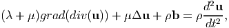 | (1.22) |
where Δ(⋅) stands for the Laplace operator and t denotes time. The detail derivation of this equation is given in chapter 7. Equation (1.22) is called the Navier-Lamè equations. Thus, in the displacement method equation (1.22) is solved along with the prescribed boundary condition.
If three dimensional solid elements are used for modeling the body in finite element programs, then the weakened form of equation (1.22) is solved for the specified boundary conditions.
In this method, the stress field is assumed such that it satisfies the equilibrium
equations as well as the prescribed traction boundary conditions. For example, in
the absence of body forces and static equilibrium, it can be easily seen that if the
Cartesian components of the stress are derived from a potential, ϕ =  (x,y,z)
called as the Airy’s stress potential as,
(x,y,z)
called as the Airy’s stress potential as,
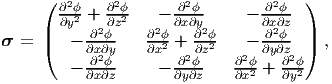 | (1.23) |
then the equilibrium equations are satisfied. Having arrived at the stress, the strain is computed using
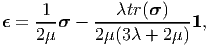 | (1.24) |
obtained by inverting the constitutive relation, (1.17). In order to be able to find a smooth displacement field from this strain, it has to satisfy compatibility condition (1.15). This procedure is formulated in chapter 7 and is followed to solve some boundary value problems in chapters 8 and 9.
This method is used to solve problems when the constitutive relation is not given by Hooke’s law (1.17). When the constitutive relation is not given by Hooke’s law, displacement method results in three coupled nonlinear partial differential equations for the displacement components which are difficult to solve. Hence, simplifying assumptions are made for the displacement field, wherein a the displacement field is prescribed but for some constants and/or some functions. Except in cases where the constitutive relation is of the form (1.16), one has to make an assumption on the components of the stress which would be nonzero for this prescribed displacement field. Then, these nonzero components of the stress field is found in terms of the constants and unknown functions in the displacement field. On substituting these stress components in the equilibrium equations and boundary conditions, one obtains differential equations for the unknown functions and algebraic equations to find the unknown constants. The prescription of the displacement field is made in such a way that it results in ordinary differential equations governing the form of the unknown functions. Since part displacement and part stress are prescribed it is called semi-inverse method. This method of solving equations would not be illustrated in this course.
Finally, we say that the boundary value problem is well posed if (1) There exist a displacement and stress field that satisfies the boundary conditions and the governing equations (2) There exist only one such displacement and stress field (3) Small changes in the boundary conditions causes only small changes in the displacement and stress fields. The boundary value problem obtained when Hooke’s law (1.17) is used for the constitutive relation is known to be well posed, as will be discussed in chapter 7.
Thus in this chapter we introduced the four concepts in mechanics, the four equations connecting these concepts as well as the methodologies used to solve boundary value problems. In the following chapters we elaborate on the same topics. It is not intended that in a first reading of this chapter, one would understand all the details. However, reading the same chapter at the end of this course, one should appreciate the details. This chapter summarizes the concepts that should be assimilated and digested during this course.