 and let 𝔄 be a set of points
in 𝔅t occupied by the particles in an arbitrary subset
and let 𝔄 be a set of points
in 𝔅t occupied by the particles in an arbitrary subset  of . If with there is
associated a non-negative real number m() having a physical dimension
independent of time and distance and such that
of . If with there is
associated a non-negative real number m() having a physical dimension
independent of time and distance and such that
The balance laws, discussed in this chapter, has to be satisfied for all bodies, irrespective of the material that they are made up of. The fundamental balance laws that would be discussed here are conservation of mass, linear momentum, and angular momentum. However, the particular form that these equations take would depend on the processes that one is interested in. Here our interest is in what is called as purely mechanical processes and hence we are not concerned about conservation of energy or electric charge or magnetic flux. These general balance equations in themselves do not suffice to determine the deformation or motion of a body subject to given loading. Also, bodies identical in geometry but made up of different material undergo different deformation or motion when subjected to the same boundary traction. Hence, to formulate a determinate problem, it is usually necessary to specify the material which the body is made. In continuum mechanics, such specification is stated by constitutive equations, which relate, for example, the stress tensor and the stretch tensor. We shall see more about these constitutive relations in the subsequent chapter while we shall focus on balance laws in this chapter.
We define a system as a particular collection of matter or a particular region of space. The complement of a system, i.e., the matter or region outside the system, is called the surroundings. The surface that separates the system from its surroundings is called the boundary or wall of the system.
A closed system consists of a fixed amount of matter in a region Ω in space with boundary surface ∂Ω which depends on time t. While no matter can cross the boundary of a closed system, energy in the form of work or heat can cross the boundary. The volume of a closed system is not necessarily fixed. If the energy does not cross the boundary of the system, then we say that the boundary is insulated and such a system is said to be mechanically and thermally isolated. An isolated system is an idealization for no physical system is truly isolated, for there are always electromagnetic radiation into and out of the system.
An open system (or control volume) focuses in on a region in space, Ωc which is independent of time t. The enclosing boundary of the open system, over which both matter and energy can cross is called a control surface, which we denote by ∂Ωc.
At the intuitive level mass is perceived to be a measure of the amount of material contained in an arbitrary portion of the body. As such it is a non-negative scalar quantity independent of time and not generally determined by the size of the configuration occupied by the arbitrary sub-body. It is not a count of the number of material particles in the body or its sub-parts. However, the mass of a body is the sum of the masses of its parts. These statements can be formalized mathematically by characterizing mass as a set function with certain properties and we proceed on the basis of the following definitions.
Let 𝔅t be an arbitrary configuration of a body and let 𝔄 be a set of points
in 𝔅t occupied by the particles in an arbitrary subset of . If with there is
associated a non-negative real number m() having a physical dimension
independent of time and distance and such that
1 ∪2) = m(1) + m(2) for all pairs 1, 2 of disjoint subsets
of , and
) → 0 as volume of A tends to zero, is said to be a material body with mass function m. The mass content of 𝔄,
denoted by m(𝔄), is identified with the mass m() of . Property two is a
consequence of our assumption that the body is a continuum, precluding the
presence of point masses. Properties (i) and (ii) imply the existence of a scalar
field ρ, defined on , such that
 | (5.1) |
ρ is called the mass density, or simply the density, of the material with which the body is made up of.
In non-relativistic mechanics mass cannot be produced or destroyed, so the mass of a body is a conserved quantity. Hence, if a body has a certain mass in the reference configuration it must stay the same during a motion. Hence, we write
 | (5.2) |
for all times t, where 𝔅r denotes the region occupied by the body in the reference configuration and 𝔅t denotes the region occupied by the body in the current configuration.
In the case of a material body executing a motion {𝔅t : t ∈ I}, the density ρ is
defined as a scalar field on the configurations {𝔅t} and the mass content m(𝔄t) of
an arbitrary region in the current configuration 𝔅t is equal to the mass m() of
. Since, m() does not depend upon t we deduce directly from (5.1) the
equation of mass balance
 | (5.3) |
ρ =  (x,t), the density is assumed to be continuously differentiable jointly in the
position and time variables on which it depends. Since, we are interested in the
total time derivative and the current volume of the body changes with time, the
differentiation and integration operations cannot be interchanged. To be able to
change the order of the integration and differentiation, we have to convert it to an
integral over the reference configuration. This is accomplished by using (3.75).
Hence, we obtain
(x,t), the density is assumed to be continuously differentiable jointly in the
position and time variables on which it depends. Since, we are interested in the
total time derivative and the current volume of the body changes with time, the
differentiation and integration operations cannot be interchanged. To be able to
change the order of the integration and differentiation, we have to convert it to an
integral over the reference configuration. This is accomplished by using (3.75).
Hence, we obtain
 | (5.4) |
Expanding the above equation we obtain
![∫
D-ρ- D-det(F)-
𝔄 [Dt det(F ) + ρ Dt ]dV = 0.
r](main600x.png) | (5.5) |
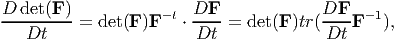
Now, we compute  . Towards this, using the chain rule for
differentiation,
. Towards this, using the chain rule for
differentiation,
 | (5.6) |
Using the result from equation (2.187),
 | (5.7) |
where to obtain the last expression we have made use of the definition of a dot product of two tensors, (2.71) and the property of the trace operator, (2.68). Defining, l = grad(v), it can be seen that
 | (5.8) |
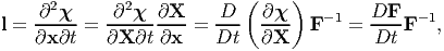
obtained using the chain rule and by interchanging the order of the spatial and temporal derivatives. Hence, equation (5.7) reduces to,
 | (5.9) |
on using the definition of the divergence, (2.208).
Substituting (5.9) in (5.5) we obtain
![∫
[D-ρ-+ ρdiv(v)]det(F )dV = 0.
𝔄r Dt](main606x.png) | (5.10) |
Again using (3.75) we obtain
![∫
D-ρ-
[Dt + ρdiv (v )]dv = 0,
𝔄t](main607x.png) | (5.11) |
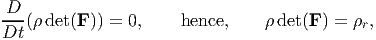
wherein the integrand is continuous in 𝔅t and the range of integration is an arbitrary subregion of 𝔅t. Since, the integral vanishes in 𝔅t and in any arbitrary subregion of 𝔅t, the integrand should vanish, i.e.,
 | (5.12) |
Subject to the presumed smoothness of ρ, equations (5.3) and (5.12) are equivalent expressions of the conservation of mass.
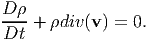
Further, since (5.4) has to hold for any arbitrary subpart of 𝔄r, we get
 | (5.13) |
where ρr is the density in the reference configuration, 𝔅r. Note that, whenever the body occupies 𝔅r, det(F) = 1 and hence, ρ = ρr, giving ρr as the constant value of ρ det(F) and hence the referential equation of conservation of mass
 | (5.14) |
A body which is able to undergo only isochoric motions is said to be composed of incompressible material. Since, det(F) = 1 for isochoric motions, we see from equation (5.14) that the density does not change with time, t. Consequently, for a body made up of an incompressible material, if the density is uniform in some configuration it has to be the same uniform value in every configuration which the body can occupy. On the other hand if a body is made up of compressible material this is not so, in general.
Let ϕ be a scalar field and u a vector field representing properties of a moving
material body, , and let 𝔄t be an arbitrary material region in the current
configuration of . Then show that:
![∫ ∫
-D- ρϕdv = -D-(ρϕ det(F ))dV,
Dt 𝔄t 𝔄rDt
∫ ( D ϕ [D ρ ] )
= ρ----+ ----+ ρdiv(v ) ϕ det(F )dV
∫𝔄r( Dt [ Dt ] )
D-ϕ- D-ρ-
= ρDt + Dt + ρdiv(v) ϕ dv, (5.17)
𝔄t](main612x.png)
There are two kinds of forces that act in a body. They are:
Contact forces arise due to contact between two bodies. Body forces are action at a distance forces like gravitational force. Similarly, while contact forces act per unit area of the boundary of the body, body forces act per unit mass of the body. Both these forces result in the generation of stresses.
Before deriving these conservation laws of momentum rigorously, we obtain the same using using an approximate analysis, as we did for the transformation of curves, areas and volumes. Moreover, we obtain these for a 2D body. Consider an 2D infinitesimal element in the current configuration with dimensions Δx along the x direction and Δy along the y direction, as shown in figure 5.1. We assume that the center of the infinitesimal element, O is located at (x + 0.5Δx,y + 0.5Δy).
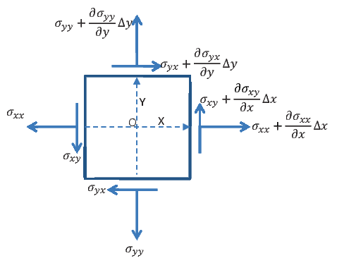
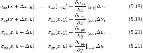
We assume that the Cauchy stress, σ varies over the infinitesimal element in
the current configuration, σ =  (x,y). That is we have assumed Eulerian
description for the stress. Since, we are considering only 2D state of stress, the
relevant Cartesian components of the stress are σxx, σyy, σxy and σyx. Expanding
the Cartesian components of the stresses using Taylor’s series up to first order we
obtain:
(x,y). That is we have assumed Eulerian
description for the stress. Since, we are considering only 2D state of stress, the
relevant Cartesian components of the stress are σxx, σyy, σxy and σyx. Expanding
the Cartesian components of the stresses using Taylor’s series up to first order we
obtain:
Now, we are interested in the equilibrium of the infinitesimal element in the deformed configuration under the action of these stresses and the body force, b with Cartesian components bx and by along the x and y direction respectively. Also, we shall assume that the infinitesimal element is accelerating with acceleration, a with Cartesian components ax and ay along the x and y direction respectively. Thus, force equilibrium along the x direction requires:
where ρ is the density and the element is assumed to have a unit thickness. Note that here ρ(Δx)(Δy)(1) gives the infinitesimal mass of the element and the stresses are multiplied by the respective areas over which they act to get the forces; since only the forces should satisfy the equilibrium equations. Simplifying, (5.22) we obtain:
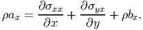 | (5.23) |
Similarly, writing the force equilibrium equation along the y direction:
The above equation simplifies to:
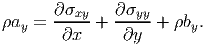 | (5.25) |
Finally, we appeal to the moment equilibrium. Here we assume that there are no body couples or contact couples acting in the infinitesimal element. Since, we can take moment equilibrium about any point, for convenience, we do it about the point O, marked in figure 5.1, to obtain:
Simplifying the above equation we obtain:
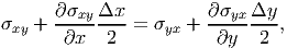 | (5.27) |
which in the limit Δx and Δy tending to zero, the limit that we are interested in, reduces to requiring
 | (5.28) |
Thus, a plane Cauchy stress field should satisfy the equations (5.23), (5.25) and (5.28) for it to be admissible.
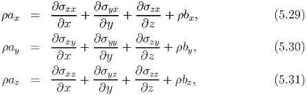
Generalizing it for 3D, the Cauchy stress field should satisfy:
and
 | (5.32) |
The equations (5.29) through (5.31) are written succinctly as
 | (5.33) |
and equations (5.32) tells us that the Cauchy stress should be symmetric.
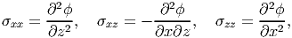
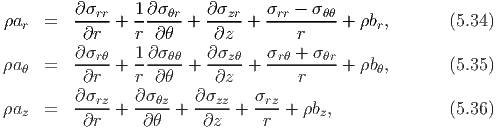
Similarly, requiring a sector of cylindrical shell to be in equilibrium, under the action of spatially varying stresses, it can be shown that
and
 | (5.37) |
has to hold.
Let 𝔄t be an arbitrary sub-region in the configuration 𝔅t of a body . The total
linear momentum, Γ(𝔄t), of the material particles occupying 𝔄t is defined
by
 | (5.38) |
Next, we find the forces acting on the body. Since, the part 𝔄t has been isolated from its surroundings, traction t(n)(x), introduced in the last chapter, acts on the boundary of the 𝔄t. In addition to traction, which arises between parts of the body that are in contact, there exist forces like gravity which act on the material particles not through contact and are called body force. The body forces are denoted by b and are defined per unit mass. Hence, the resultant force, г acting on 𝔄t is
 | (5.39) |
Now, using Newton’s second law of motion, which states that the rate of change of linear momentum of the body must equal the resultant force that acts on the body in both magnitude and direction we obtain
 | (5.40) |
Using (3.30), definition of acceleration, a and (5.16) the above equation can be written as
 | (5.41) |
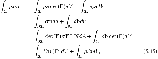
Next, using Cauchy’s stress theorem (4.3) and the divergence theorem (2.263) the above equation further can be reduced to
![∫ ∫ ∫ ∫
ρadv = σnda + ρbdv = [div(σ) + ρb ]dv.
𝔄t ∂𝔄t 𝔄t 𝔄t](main632x.png) | (5.42) |
Since, the above equation has to hold for 𝔅t and any subset, 𝔄t, of it
 | (5.43) |
Many a times, we are interested in cases for which a = o, then (5.43) becomes
 | (5.44) |
which is referred to as Cauchy’s equation of equilibrium. Further, there arises scenarios where the body forces can be neglected and in those cases div(σ) = o. Thus, divergence free stress fields are called self equilibrated stress fields.
Equation (5.43) is in spatial form, that is it assumes that σ =  (x,t), b =
 (x,t), a =
  (x,t), ρ =
  (x,t) are known. But on most occasions, especially in
solid mechanics, we know only the material form of these fields that is σ =
(x,t) are known. But on most occasions, especially in
solid mechanics, we know only the material form of these fields that is σ =
 (X,t), b =
  (X,t), a =
  (X,t), ρ =
  (X,t) and in those occasions it is difficult
to obtain the spatial divergence of these fields. To make it easier at these
instances, we seek a statement of balance of linear momentum in material form.
For this, equation (5.42a) has to be modified. Towards this, we obtain
(X,t) and in those occasions it is difficult
to obtain the spatial divergence of these fields. To make it easier at these
instances, we seek a statement of balance of linear momentum in material form.
For this, equation (5.42a) has to be modified. Towards this, we obtain
 | (5.46) |
It is worthwhile to emphasize that irrespective of the choice of the independent variable, the equilibrium of the forces is established only in the current configuration. In other words, whether we use material or spatial description for the stress, the forces and moments have to be equilibrated in the deformed configuration and not the reference configuration.
Let 𝔄t be an arbitrary sub-region in the configuration 𝔅t of a body . The total
angular momentum, Ω(𝔄t), of the material particles occupying 𝔄t is defined
by
![∫
Ω (𝔄 ) = [(x - x ) ∧ ρv + p]dv,
t 𝔄t o](main645x.png) | (5.47) |
where xo is the point about which the moment is taken and p is the intrinsic angular momentum per unit volume in the current configuration.
Next, we find the moment due to the forces acting on the body. As discussed
before there are two kind of forces, surface or contact forces and body forces
act on the body which contribute to the moment. Apart from moment
arising due to applied forces, there could exist couples distributed per unit
surface area, m and body couples c, defined per unit mass. Thus, m =
 (x,t,n) and c =
  (x,t). Hence, the resultant moment, ω acting on 𝔄t
is
(x,t). Hence, the resultant moment, ω acting on 𝔄t
is
![∫ ∫
ω(𝔄t ) = [(x - xo) ∧ t(n ) + m ]da + [ρ(x - xo) ∧ b + c]dv.
∂𝔄t 𝔄t](main648x.png) | (5.48) |
However, in non-polar bodies that are the subject matter of the study here, there exist no body couples or couples distributed per unit surface area or intrinsic angular momentum, i.e., c = m = p = o.
The balance of angular momentum states that the rate of change of the angular momentum must equal the applied momentum in both direction and magnitude. Hence,
 | (5.49) |
Further simplification of this balance principle involves some tensor algebra. First, we begin by calculating the left hand side of the above equation:
Since, v ∧ v = o and using equations (5.13) and (5.9), (5.50) reduces toNext, we simplify the right hand side of the equation (5.49). Towards that, we first show that
![∫ ∫
(x - xo) ∧ σtnda = [(x - xo) ∧ div(σ) - τ ]dv,
∂𝔄t 𝔄t](main652x.png) | (5.52) |
where τ is the axial vector of (σ - σt). We begin by establishing a few vector identities which enable us to establish (5.52).
Identity - 1: If u and v are arbitrary vectors then u ∧ v is the axial vector of the skew-symmetric tensor v ⊗ u - u ⊗ v.
Proof: It is straightforward to verify that v ⊗ u - u ⊗ v is skew-symmetric. Then we observe that
 | (5.53) |
hence, the axial vector of v ⊗ u - u ⊗ v is a scalar multiple of u ∧ v. Accordingly,
 | (5.54) |
for any vector a. Now, we have to show that α = 1. Setting a = u in the above equation and then forming a scalar product on each side with v we have
 | (5.55) |
Using (2.36) we find that
![α{(u ∧ v ) ∧ u} ⋅ v = α[(u ⋅ u)(v ⋅ v) - (u ⋅ v)2].](main656x.png) | (5.56) |
Comparing equations (5.55) and (5.56) we find that α = 1.
Identity - 2: For any vector a, b, c in the vector space
 | (5.57) |
This identity follows immediately from the above identity.
Identity - 3: Let 𝔄t be a regular region with boundary ∂𝔄t, let n be the outward unit normal to ∂𝔄t and let u be a vector field and σ a tensor field, each continuous in 𝔄t and continuously differentiable in the interior of 𝔄t. Then
 | (5.58) |
Towards proving this identity, note that
where a is an arbitrary constant vector. To obtain the above we have made use of the identities
![∫ ∫
σn ⊗ uda = [div(σ) ⊗ u + σt{grad (u)}t]dv
∂𝔄t 𝔄t](main661x.png) | (5.62) |
Taking the transpose of the above identity, we obtain the required vector identity (5.58).
Now, we are in a position to prove (5.52). For this we replace b by (x - xo) and c by σn in (5.57) and then integrating each side over the surface ∂𝔄t we obtain
 | (5.63) |
a being an arbitrary vector. From (5.58) it follows that
![∫ ∫
a ∧ (x - x ) ∧ (σn )da = {[(x - x ) ⊗ div(σ) - div(σ ) ⊗ (x - x )]a
∂𝔄t o 𝔄t o o
t
+ (σ - σ )a }dv (5.66 )](main664x.png)
![∫ ∫
a ∧ (x - xo) ∧ (σn )da = a ∧ [(x - xo ) ∧ div(σ ) - τ ]dv,
∂𝔄t 𝔄t](main665x.png) | (5.67) |
and hence the required identity (5.52), since a is an arbitrary vector.
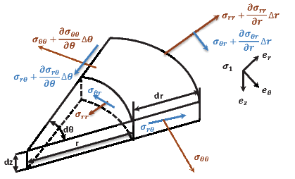
Substituting (5.51) and (5.52) in (5.49) yields
![∫ ∫
mda = [(x - xo) ∧ (ρa - div(σ ) - ρb)]dv
∂𝔄t 𝔄t ∫
+ [Dp--+ pdiv (v) - c + τ]dv. (5.68)
𝔄t Dt](main666x.png)
![∫ ∫
mda = [Dp--+ pdiv (v) - c + τ]dv.
∂𝔄t 𝔄t Dt](main667x.png) | (5.69) |
Here we are interested only in non-polar bodies and hence, p = c = m = o. Therefore, (5.69) simplifies to requiring
 | (5.70) |
Since, this has to hold for any arbitrary subparts of the body, 𝔅t, τ = o. Consequently,
 | (5.71) |
that is the Cauchy stress tensor has to be symmetric in non-polar bodies.
Since, in this course we are interested only in purely mechanical process, we studied only conservation of mass and momentum. There are other quantities like energy, charge which is also conserved. In courses on thermodynamics or electromagnetism, one would study the other conservation laws. The one equation that would be used frequently in the following chapters is the final expression for the conservation of linear momentum, also called as equilibrium equations,
 | (5.72) |
where ρ is the density, b is the body force per unit mass, σ is the Cauchy stress tensor.
 |
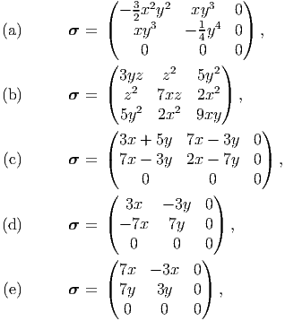
Find the body force that should act on the plate so that this state of stress is realizable in the body.
 |
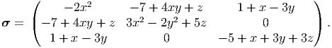
where ϕ = (x,y), for any choice of ϕ. ϕ is called the Airy’s stress potential.
 |

![[ ]
ρ(Δx )(Δy )(1 )a = σ (x, y) + ∂σxx| Δx - σ (x,y) (Δy )(1)
x xx ∂x (x,y) xx
[ ∂σ ]
+ σyx(x,y) + ---yx-|(x,y)Δy - σyx(x,y) (Δx )(1)
∂y
+ρ(Δx )(Δy )(1)bx, (5.22)](main616x.png)
![[ ]
∂σxy
ρ(Δx )(Δy )(1 )ay = σxy(x, y) + -∂x-|(x,y)Δx - σxy (x, y) (Δy )(1)
[ ]
∂σyy-
+ σyy(x,y) + ∂y |(x,y)Δy - σyy(x,y) (Δx )(1)
+ρ (Δx )(Δy )(1)by. (5.24)](main618x.png)
![[ ]
σ (x, y) + σ (x, y) + ∂σxy| Δx (Δx-) (Δy )(1)
xy xy ∂x (x,y) 2
[ ∂σ ] (Δy )
= σyx(x, y) + σyx (x, y) +--yx|(x,y)Δy -----(Δx )(1).(5.26)
∂y 2](main620x.png)
![[∫ ]
D Ω D
---- = --- [(x - xo) ∧ ρv + p]dv
Dt D∫t 𝔄t
D--
= 𝔄 Dt { [(x - xo) ∧ ρv + p ]det(F)} dV
∫ r { }
= v ∧ ρv det(F) + (x - xo) ∧ -D-(ρ det(F))v + ρa det(F ) dV
𝔄r Dt
∫ D
+ ---(p det(F ))dV. (5.50)
𝔄rDt](main650x.png)
![[ ]
D Ω ∫ ∫ Dp
---- = [(x - xo) ∧ ρa]det(F )dV + ----+ pdiv(v) det(F)dV
Dt ∫𝔄r{ 𝔄r D}t
Dp--
= [(x - xo ) ∧ ρa] + Dt + pdiv (v) dv. (5.51)
𝔄t](main651x.png)
![∫ ∫ ∫
(σn ⊗ u )ada = (u ⋅ a)σnda = div((u ⋅ a)σ)dv
∂𝔄t ∫∂𝔄t 𝔄t
= [(u ⋅ a )div (σ ) + σtgrad (u ⋅ a)dv
𝔄t
∫
= [div(σ ) ⊗ u + σt{grad (u)}t]adv (5.59)
𝔄t](main659x.png)