Mechanics is the branch of science that describes or predicts the state of rest or of motion of bodies subjected to some forces. In the last chapter, we studied about mathematical descriptors of the state of rest or of motion of bodies. Now, we shall focus on the cause for motion or change of geometry of the body; the force. While in rigid body mechanics, the concept of force is sufficient to describe or predict the motion of the body, in deformable bodies it is not. For example, two bars made of the same material and of same length but with different cross sectional area, will undergo different amount of elongation when subjected to the same pulling force acting parallel to the axis of the bar. It was then found that if we define a quantity called strain which is defined as the ratio between the change in length to the original length of the bar along the direction of the applied load and a quantity called stress which is defined as the force acting per unit area then the stress and strain could be related through an equation that is independent of the geometry of the body but depend only on the material that the body is made up of. While these definitions of strain and stress are adequate to study homogeneous deformations resulting from uniform stress states, these concepts have to be generalized to study the motion of bodies subjected to a non-uniform distribution of forces and/or couples. In this chapter, we shall generalize the concept of stress having already generalized the concept of strain in the last chapter.
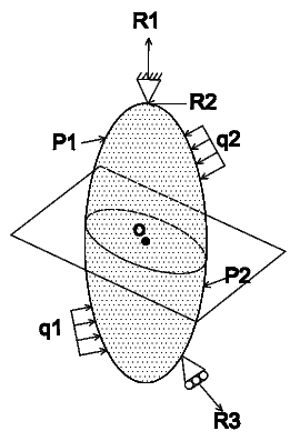
Here we focus attention on a deformable continuum body  occupying an
arbitrary region 𝔅t of the Euclidean vector space with boundary surface ∂𝔅t at
time t, as shown in figure 4.1a. We consider a general case where in arbitrary
forces act on parts or the whole of the boundary surface called the external forces
or loads. Recognizing that these external forces arose because we isolated
the body from its surroundings, to find the internal forces we have to
section the body. Thus, to find the internal forces on a internal surface
passing through O, as indicated in the figure 4.1a, we have to section
the body as shown in the figure 4.1b, with the cutting plane coinciding
with the internal surface. Now, we focus our attention on an infinitesimal
part of the body centered around O, see figure 4.2. Let x be the position
vector of the point O, n a unit vector directed along the outward normal
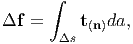
to an infinitesimal spatial surface element Δs, at x and Δf denote the
infinitesimal resultant force acting on the surface element Δs. Then, we claim
that
occupying an
arbitrary region 𝔅t of the Euclidean vector space with boundary surface ∂𝔅t at
time t, as shown in figure 4.1a. We consider a general case where in arbitrary
forces act on parts or the whole of the boundary surface called the external forces
or loads. Recognizing that these external forces arose because we isolated
the body from its surroundings, to find the internal forces we have to
section the body. Thus, to find the internal forces on a internal surface
passing through O, as indicated in the figure 4.1a, we have to section
the body as shown in the figure 4.1b, with the cutting plane coinciding
with the internal surface. Now, we focus our attention on an infinitesimal
part of the body centered around O, see figure 4.2. Let x be the position
vector of the point O, n a unit vector directed along the outward normal
to an infinitesimal spatial surface element Δs, at x and Δf denote the
infinitesimal resultant force acting on the surface element Δs. Then, we claim
that
 | (4.1) |
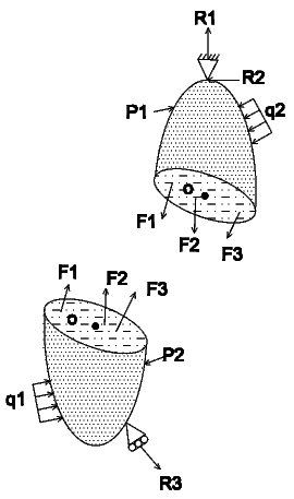
where t(n) =  (x,t,n) represents the Cauchy (or true) traction vector and the
integration here denotes an area integral. Thus, Cauchy traction vector is the
force per unit surface area defined in the current configuration acting at a given
location. The Cauchy traction vector and hence the infinitesimal force at a given
location depends also on the orientation of the cutting plane, i.e., the unit
normal n. This means that the traction and hence the infinitesimal force
at the point O, for a vertical cutting plane could be different from that
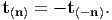
of a horizontal cutting plane. However, the traction on the two pieces
of the cut body would be such that they are equal in magnitude but
opposite in direction, in order to satisfy Newton’s third law of motion.
Hence,
(x,t,n) represents the Cauchy (or true) traction vector and the
integration here denotes an area integral. Thus, Cauchy traction vector is the
force per unit surface area defined in the current configuration acting at a given
location. The Cauchy traction vector and hence the infinitesimal force at a given
location depends also on the orientation of the cutting plane, i.e., the unit
normal n. This means that the traction and hence the infinitesimal force
at the point O, for a vertical cutting plane could be different from that
of a horizontal cutting plane. However, the traction on the two pieces
of the cut body would be such that they are equal in magnitude but
opposite in direction, in order to satisfy Newton’s third law of motion.
Hence,
 | (4.2) |
This requires:  (x,t,n) = -
 (x,t,-n).
Relationship (4.1) is referred to as Cauchy’s postulate. It is worthwhile to mention that in any experiment we infer only these traction vectors. In literature, the traction vector is also called as stress vector because they have the units of stress, i.e., force per unit area. However, here we shall not use this terminology and for us stress is always a tensor, as defined next.
There exist unique second order tensor field σ, called the Cauchy (or true) stress tensor, so that
 | (4.3) |
where σ =  (x,t) =
  (X,t), X ∈𝔅r, is the position vector of the material
particle in the reference configuration. It is easy to verify that the requirement
(4.2) is met by (4.3). It will be shown in the next chapter that the Cauchy stress
tensor, σ has to be a symmetric tensor. However, the proof of Cauchy stress
theorem is beyond the scope of these lecture notes.
(X,t), X ∈𝔅r, is the position vector of the material
particle in the reference configuration. It is easy to verify that the requirement
(4.2) is met by (4.3). It will be shown in the next chapter that the Cauchy stress
tensor, σ has to be a symmetric tensor. However, the proof of Cauchy stress
theorem is beyond the scope of these lecture notes.
It is recalled that only traction vector can be determined or inferred in the experiments and hence the components of the stress tensor is estimated from finding the traction vector on three (mutually perpendicular) planes. Let us see how.
The components of the Cauchy stress tensor, σ with respect to an orthonormal basis {ea} is given by:
 | (4.4) |
In view of Cauchy’s theorem t(ea) = σte a, a = 1, 2, 3, characterize the three traction vectors acting on the surface elements whose outward normals point in the directions e1, e2, e3, respectively. Then, the components of these traction vectors along e1, e2, e3 gives the various components of the stress tensor. Thus, for each stress component σab we adopt the mathematically logical convention that the index b characterizes the component of the traction vector, t(ea), at a point x in the direction of the associated base vector eb and the index a characterizes the orientation of the area element on which t(n) is acting.
It is important to note that some authors reverse this convention by identifying the index b with the orientation of the normal to the plane of cut and the index a with the component of the traction along the direction ea. Irrespective of the convention adopted the end results will be the same because of two reasons: (i) The definition of divergence is suitably modified with a transpose (ii) the Cauchy stress tensor is anyway symmetric.
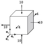
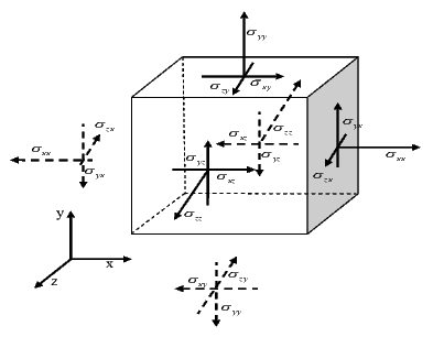
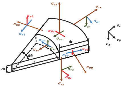
In other words, to find the components of the Cauchy stress tensor, at a given location, we isolate an infinitesimal cube with the location of interest at its center. The cube is oriented such that the outward normal to its sides is along or opposite to the direction of the basis vectors. Hence, for general curvilinear coordinates, the sides of the cube need not be plane nor make right angles with each other. Compare the stress cube for Cartesian basis (figure 4.3) and cylindrical polar basis (figure 4.4). Then, we determine the traction that is acting on each of the six faces of the cube. Due to equation (4.2) only three of these six traction vectors are independent. The components of the three traction vectors along the the three basis vectors gives the nine components of the stress tensor.
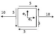
If the component of the traction is along the direction of the basis vectors on planes whose outward normal coincides with the direction of the basis vectors it is considered to be positive and negative otherwise. Consistently, if the component of the traction is opposite to the direction of the basis vectors on faces of the cube whose outward normal is opposite in direction to the basis vectors, it is considered to be positive and negative otherwise. Thus, one should not be confused that the same stress component points in opposite directions on opposite planes. This is necessary for the cube under consideration to be in equilibrium. It should also be appreciated that the sign of some of the stress component does change when the direction of the coordinate basis is reversed even if the right handedness of the basis vectors is maintained. This is so, because the sign of the stress component depends both on the direction of coordinate basis as well as the outward normal. Thus, figure 4.3 portrays the positive components of the stress tensor when Cartesian coordinate basis is used and it is called as the stress cube.
The positive cylindrical polar components of the stress tensor is depicted on a cylindrical wedge in figure 4.4. Recognize that the direction of the cylindrical polar components of the stress changes with the location unlike the Cartesian coordinate components whose directions are fixed. This happens because the direction of the cylindrical polar coordinate basis vectors depends on the location. Here σrr component of the stress is called as the radial stress, σθθ component of the stress is known as the hoop or the circumferential stress, σzz component of the stress is the axial stress.
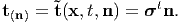
Let the traction vector t(n) for a given current position x at time t act on an arbitrarily oriented surface element characterized by an outward unit normal vector n.
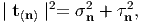
The traction vector t(n) may be resolved into the sum of a vector along the normal n to the plane, denoted by t(n)∥ and a vector perpendicular to n denoted by t(n)⊥, i.e., t (n) = t(n)∥ + t (n)⊥. From the results in section 2.3.3, it could be seen that
where It could easily be verified that n ⋅ m = 0. This means m is a vector embedded in the surface. Then, σn is called the normal traction and τn is called the shear traction. As the names suggest, normal traction acts perpendicular to the surface and shear traction acts tangential or parallel to the surface.Since, t(n) = t(n)∥ + t (n)⊥, we obtain the useful relation
 | (4.9) |
where we have made use of the property that n ⋅ m = 0.
It could be seen from figure 4.3 that the stress components corresponding to Cartesian basis, σxx, σyy and σzz act normal to their respective surfaces and hence are called normal stresses and the remaining independent components, σxy, σyz and σzx act parallel to the surface and hence are called shear stresses. (Remember that Cauchy stress is a symmetric tensor.) When the stress components are determined with respect to any coordinate basis vectors, there will be three normal stresses corresponding to σii and three shear stresses, σij, i≠j. Here to call certain components of the stresses as normal and others as shear, we have exploited the relationship between the components of the stress tensor and the traction vector.
At a given location in the body the magnitude of the normal and shear traction depend on the orientation of the plane. An isotropic body can fail along any plane and hence we require to find the maximum magnitude of these normal and shear traction and the planes for which these occur. As we shall see on planes where the maximum or minimum normal stresses occur the shear stresses are zero. However, in the plane on which maximum shear stress occurs, the normal stresses will exist.
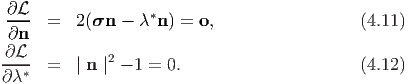
In order to obtain the maximum and minimum values of σn, the normal traction, we have to find the orientation of the plane in which this occurs. This is done by maximizing (4.5) subject to the constraint that ∣n∣ = 1. This constrained optimization is done by what is called as the Lagrange-multiplier method. Towards this, we introduce the function
![L(n, λ*) = n ⋅ σn - λ*[| n |2 - 1],](main527x.png) | (4.10) |
where λ* is the Lagrange multiplier and the condition ∣n∣2 - 1 = 0 characterizes
the constraint condition. At locations where the extremal values of  occurs, the
derivatives
occurs, the
derivatives  and
and  must vanish, i.e.,
 a and λa*’s such
that
a and λa*’s such
that
 | (4.13) |
(a = 1, 2, 3; no summation) which is nothing but the eigenvalue problem involving the tensor σ with the Lagrange multiplier being identified as the eigenvalue. Hence, the results of section 2.5 follows. In particular, for (4.13a) to have a non-trivial solution
 | (4.14) |
where
![K1 = tr(σ), K2 = 1[K2 - tr(σ2 )], K3 = det (σ ),
2 1](main534x.png) | (4.15) |
the principal invariants of the stress σ. As stated in section 2.5, equation (4.14) has three real roots, since the Cauchy stress tensor is symmetric. These roots (λa*) will henceforth be denoted by σ 1, σ2 and σ3 and are called principal stresses. The principal stresses include both the maximum and minimum normal stresses among all planes passing through a given x.
The corresponding three orthonormal eigenvectors  a, which are then
characterized through the relation (4.13) are called the principal directions of σ.
The planes for which these eigenvectors are normal are called principal planes.
Further, these eigenvectors form a mutually orthogonal basis since the stress
tensor σ is symmetric. This property of the stress tensor also allows us to
represent σ in the spectral form
a, which are then
characterized through the relation (4.13) are called the principal directions of σ.
The planes for which these eigenvectors are normal are called principal planes.
Further, these eigenvectors form a mutually orthogonal basis since the stress
tensor σ is symmetric. This property of the stress tensor also allows us to
represent σ in the spectral form
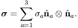 | (4.16) |
It is immediately apparent that the shear stresses in the principal planes are zero. Thus, principal planes can also be defined as those planes in which the shear stresses vanish. Consequently, σa’s are normal stresses.
Next, we are interested in finding the direction of the unit vector n at x that gives the maximum and minimum values of the shear traction, τp. This is important because in many metals the failure is due to sliding of planes resulting due to the shear traction exceeding a critical value along some plane.
In the following we choose the eigenvectors { a} of σ as the set of basis
vectors. Then, according to the spectral decomposition (4.16), all the
non-diagonal matrix components of the Cauchy stress vanish. Then, the traction
vector t(p) on an arbitrary plane with normal p could simply be written
as
a} of σ as the set of basis
vectors. Then, according to the spectral decomposition (4.16), all the
non-diagonal matrix components of the Cauchy stress vanish. Then, the traction
vector t(p) on an arbitrary plane with normal p could simply be written
as
 | (4.17) |
where p = p1 1 + p2
 2 + p3
 3. It then follows from (4.9) that
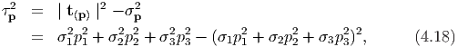
With the constraint condition ∣p∣2 = 1 we can eliminate p 3 from the equation (4.18). Then, since the principal stresses, σ1, σ2, σ3 are known, τp2 is a function of only p1 and p2. Therefore to obtain the extremal values of τp2 we differentiate τ p2 with respect to p 1 and p2 and equate it to zero1 :
![∂τ2
--p-= 2p1[σ1 - σ3 ]{σ1 - σ3 - 2[(σ1 - σ3)p21 + (σ2 - σ3)p22]} = 0, (4.19)
∂p1
∂ τ2p 2 2
---- = 2p2[σ2 - σ3]{σ2 - σ3 - 2[(σ1 - σ3)p1 + (σ2 - σ3)p2]} = 0. (4.20)
∂p2](main543x.png)
 and hence p3 = ±1∕
 .
.
 , p2 = 0 and hence p3 = ±1∕
 .
.Instead of eliminating p3 we could eliminate p2 or p1 initially and find the remaining unknowns by adopting a procedure similar to the above. Then, we shall find the extremal values of τp could also occur when
 and hence p2 = ±1∕
 .
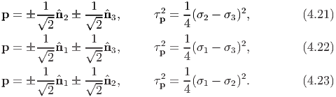
.Substituting these solutions in (4.18) we find the extremal values of τp. Thus, τp = 0
when p = ± 1 or p = ±
 2 or p = ±
 3 and
3 and
Consequently, the maximum magnitude of the shear traction denoted by τmax is given by the largest of the three values of (4.21b) - (4.23b). Thus, we obtain
 | (4.24) |
where σmax and σmin denote the maximum and minimum magnitudes of principal stresses, respectively. Recognize that the maximum shear stress acts on a plane that is shifted about an angle of ±45 degrees to the principal plane in which the maximum and minimum principal stresses act. In addition, we can show that the normal traction σp to the plane in which τmax occurs has the value σp = (σmax + σmin)∕2.
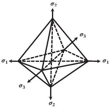
Consider now a tetrahedron element similar to that of figure 4.5 with a plane equally inclined to the principal axes. Hence, its normal is given by
 | (4.25) |
where  a are the three principal directions of the Cauchy stress tensor. Then, the
normal traction, σoct, on this plane is
a are the three principal directions of the Cauchy stress tensor. Then, the
normal traction, σoct, on this plane is
![1
σoct = -[σ1 + σ2 + σ3 ],
3](main558x.png) | (4.26) |
obtained using (4.5) and the spectral representation for the Cauchy stress (4.16). Similarly, the shear traction, τoct on this plane is
![1 1
τ2oct = -[σ21 + σ22 + σ23] - -(σ1 + σ2 + σ3)2.
3 9](main559x.png) | (4.27) |
From the definition of principal invariants for stress (4.15) it is easy to verify that
 | (4.28) |
Using the above formula one can compute the octahedral normal and shear traction for stress tensor represented using some arbitrary basis.
Specifying a state of stress means providing sufficient information to compute the components of the stress tensor with respect to some basis. As discussed before, knowing t(n) for three independent pairs of {t(n),n} we can construct the stress tensor σ. Hence, specifying the set of pairs {(t(n),n)} for three independent normal vectors, n, at a given point, so that the stress tensor could be uniquely determined tantamount to prescribing the state of stress. Next, we shall look at some states of stress.
The state of stress is said to be uniform if the stress tensor does not depend on the space coordinates at each time t, when the stress tensor is represented using Cartesian basis vectors.
If the stress tensor has a representation
 | (4.29) |
at some point, where n is a unit vector, we say it is in a pure normal stress state. Post-multiplying (4.29) with the unit vector n we find that
 | (4.30) |
Evidently, the traction is along (or opposite to) n. This stress σ characterizes either pure tension (if σ > 0) or pure compression (if σ < 0).
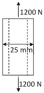
If we have a uniform stress state and the stress tensor when represented using a Cartesian basis is such that σxx = σ = const and all other stress components are zero, then such a stress state is referred to as uniaxial tension or uniaxial compression depending on whether σ is positive or negative respectively. This may be imagined as the stress in a rod with uniform cross-section generated by forces applied to its plane ends in the x - direction. However, recognize that this is not the only system of forces that would result in the above state of stress; all that we require is that the resultant of a system of forces should be oriented along the ex direction.
If the stress tensor has a representation
 | (4.31) |
at any point, where n and m are unit vectors such that n ⋅ m = 0, then it is said to be in equibiaxial stress state.
On the other hand, if the stress tensor has a representation
 | (4.32) |
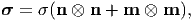
at any point, where n and m are unit vectors such that n ⋅ m = 0, then it is said to be in pure shear stress state. Post-multiplying (4.32) with the unit vector n we obtain
![σn = τ(n ⊗ m + m ⊗ n )n
= τ[(m ⋅ n)n + (n ⋅ n)m ] = τm = t⊥m. (4.33)](main565x.png)
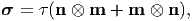
More generally, if the stress tensor has a representation
 | (4.34) |
at any point, where n and m are unit vectors such that n ⋅ m = 0, then it is said to be in plane or biaxial state of stress. That is in this case one of the principal stresses is zero. A general matrix representation for the stress tensor corresponding to a plane stress state is:
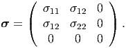 | (4.35) |
Here we have assumed that e3 is a principal direction and that there exist no stress components along this direction. We could have assumed the same with respect to any one of the other basis vectors. A plane stress state occurs at any unloaded surface in a continuum body and is of practical interest.
Next, we consider 3D stress states. Analogous to the equibiaxial stress state in 2D, if the stress tensor has a representation
 | (4.36) |
at some point, we say that it is in a hydrostatic state of stress and p is called as hydrostatic pressure. It is just customary to consider compressive hydrostatic pressure to be positive and hence the negative sign. Post-multiplying (4.36) by some unit vector n, we obtain
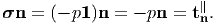 | (4.37) |
Thus, on any surface only normal traction acts, which is characteristic of (elastic) fluids at rest that is not able to sustain shear stresses. Hence, this stress is called hydrostatic.
Any other state of stress is called to be triaxial stress state.
Many a times the stress is uniquely additively decomposed into two parts namely an hydrostatic component and a deviatoric component, that is
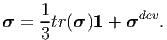 | (4.38) |
Thus, the deviatoric stress is by definition,
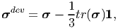 | (4.39) |
and has the property that tr(σdev) = 0. Physically the hydrostatic component of the stress is supposed to cause volume changes in the body and the deviatoric component cause distortion in the body. (Shear deformation is a kind of distortional deformation.)
Till now, we have been looking only at the Cauchy (or true) stress. As its name suggest this is the “true” measure of stress. However, there are many other definition of stresses but all of these are propounded just to facilitate easy algebra. Except for the first Piola-Kirchhoff stress, other stress measures do not have a physical interpretation as well.
Let ∂Ωt denote some surface within or on the boundary of the body in the current configuration. Then, the net force acting on this surface is given by
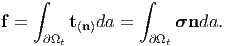 | (4.40) |
It is easy to compute the above integral when the Cauchy stress is expressed as a
function of x, the position vector of a typical material point in the current
configuration, i.e. σ =  (x,t). On the other hand computing the above integral
becomes difficult when the stress is a function of X, the position vector of a
typical material point in the reference configuration, i.e. σ =
(x,t). On the other hand computing the above integral
becomes difficult when the stress is a function of X, the position vector of a
typical material point in the reference configuration, i.e. σ =  (X,t). To facilitate
the computation of the above integral in the later case, we appeal to the Nanson’s
formula (3.72) to obtain
(X,t). To facilitate
the computation of the above integral in the later case, we appeal to the Nanson’s
formula (3.72) to obtain
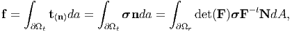 | (4.41) |
where ∂Ωr is the surface in the reference configuration, formed by the same material particles that formed the surface ∂Ωt in the current configuration. Then, the first Piola-Kirchhoff stress, P is defined as
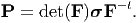 | (4.42) |
Using this definition of Piola-Kirchhoff stress, equation (4.41) can be written as
 | (4.43) |
Assuming, the stress to be uniform over the surface of interest and the state of stress corresponds to pure normal stress, it is easy to see that while Cauchy stress is force per unit area in the current configuration, Piola-Kirchhoff stress is force per unit area in the reference configuration. This is the essential difference between the Piola-Kirchhoff stress and Cauchy stress. Recognize that in both the cases the force acts only in the current configuration. In lieu of this Piola-Kirchhoff stress is a two-point tensor, similar to the deformation gradient, in that it is a linear transformation that relates the unit normal to the surface in the reference configuration to the traction acting in the current configuration. Thus, if {Ea} denote the three Cartesian basis vectors used to describe the reference configuration and {ea} denote the Cartesian basis vectors used to describe the current configuration, then the Cauchy stress and Piola-Kirchhoff stress are represented as
 | (4.44) |
We had mentioned earlier that the Cauchy stress tensor is symmetric for reasons to be discussed in the next chapter. Since, σ = PFt∕ det(F), the symmetric restriction on Cauchy stress tensor requires the Piola-Kirchhoff stress to satisfy the relation
 | (4.45) |
Consequently, in general P is not symmetric and has nine independent components.
During an experiment, it is easy to find the surface areas in the reference configuration and determine the traction or forces acting on these surfaces as the experiment progresses. Thus, Piola-Kirchhoff stress is what could be directly determined. Also, it is the stress that is reported, in many cases. The Cauchy stress is then obtained using the equation (4.42) from the estimate of the Piola-Kirchhoff stress and the deformation of the respective surface.
Further, since in solid mechanics, the coordinates of the material particles in the reference configuration is used as independent variable, first Piola-Kirchhoff stress plays an important role in formulating the boundary value problem as we shall see in the ensuing chapters.
The transpose of the Piola-Kirchhoff stress, Pt, is called as engineering stress or nominal stress.
Another stress measure called the second Piola-Kirchhoff stress, S defined as
 | (4.46) |
is used in some studies. Note that this tensor is symmetric and hence its utility.
Next, we define a few stress measures popular in literature. It is easy to establish their inter-relationship and properties which we leave it as an exercise.
The Kirchhoff stress tensor, τ is defined as: τ = det(F)σ.
The Biot stress tensor, TB also called material stress tensor is defined as: TB = RtP, where R is the orthogonal tensor obtained during polar decomposition of F.
The co-rotated Cauchy stress tensor σu, introduced by Green and Naghdi is defined as: σu = RtσR.
The Mandel stress tensor, used often to describe inelastic response of materials is defined as Σ = CS, where C is the right Cauchy-Green stretch tensor introduced in the previous chapter.
In this chapter, we introduced the concept of traction and stress tensor. If the forces acting in the body are assumed to be distributed over the surfaces in the current configuration of the body, then the corresponding traction is called as Cauchy traction and the stress tensor associated with this traction is called as the Cauchy stress tensor, σ. Similarly, if the forces acting in the body is distributed over the surface in the reference configuration, then this traction is called as Piola traction and the stress tensor associated with this traction the Piola-Kirchhoff stress, P. We also defined various types of stresses like normal stress, shear stress, hydrostatic stress, octahedral stress. Having grasped the concepts of strain and stress we shall proceed to find the relation between the applied force and realized displacement in the following chapters.
 |
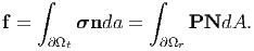
For this stress state,
 .
.
 x,
x, y,
y, z}. The new basis is obtained by rotating an angle 30
degrees in the clockwise direction about ez axis.
z}. The new basis is obtained by rotating an angle 30
degrees in the clockwise direction about ez axis.
 |
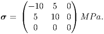
For this stress state solve parts (a) through (n) in problem 1.
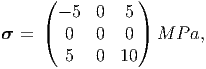 |
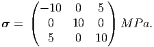
where the components of the stress is with respect to an orthonormal Cartesian basis ({ex,ey,ez}). For this state of stress, answer the following:
![t∥(n) = [n ⋅ t(n)]n = [n ⋅ σn ]n = σnn, (4.5)
⊥
t(n) = t(n) - [n ⋅ t(n)]n = [1 - n ⊗ n ]t(n) = τnm, (4.6)](main524x.png)
![τn = | t(n) - [n ⋅ t(n)]n |= | σn - [n ⋅ σn ]n |, (4.7)
-1-
m = τ {t (n) - [n ⋅ t(n)]n}. (4.8)
n](main525x.png)