Solution of one dimensional advection-diffusion equation
The one-dimensional advection diffusion equation can be written as
![]() (40.45)
(40.45)
The finite difference approximation of the equation (40.45) can be written as,
![]() (40.46)
(40.46)
Rearranging,
![]() (40.47)
(40.47)
The equation (40.47) can be used to obtain the spatial and temporal distribution of concentration iteratively. For the boundary and initial conditions given in equations (40.2), (40.3) and (40.4), solution of the two dimensional advection diffusion equation can be obtained using the following Matlab code.
![Text Box: clear all; % Define the input parameters miu = 0.5; sigma = 0.07; D=0.0005; % sqm/day v=0.005; %in m/day L =1.0; % in m delx = 0.008;% in m delt = 0.05; % in m %%%%%%%%%%%%%%%%%%%%%%%%%%%%% x = 0:delx:L; % Spatial discretization of the domain t=0:delt:10; % Time discretization of the domain [mx nx]=size(x); % Size of x [mt nt]=size(t); % Size of t C = zeros(nx,nt); % Initializing C % Initial condition: Normally distributed concentration for i=2:nx-1 C(i,1) = (1/sqrt(2*pi*sigma^2))*exp(-(x(i)-miu)^2/(2*sigma^2)) ; end C1=max(max(C)); % Main finite difference iteration for n=2:nt for i=2:nx-1 C(i,n) = C(i,n-1)+((D*delt)/delx^2)*(C(i+1,n-1)-2*C(i,n-1)+C(i-1,n-1))-(v*delt/(2*delx))*(C(i+1)-C(i-1)); end end C=C/C1; % Generating concentration distribution plot hold on; for t=1:25:nt plot(x,C(:,t), 'color',[rand rand rand]); end axis tight; xlabel('Normalized distance'); ylabel('C/Co'); M=delt*(1:25:nt); M = num2str(M'); legend(M); %%%%%%%%%%% END %%%%%%%%%%%%%%%%%%%%%%%%%%%%%%%](images/027.png)
Solutions obtained using the code are shown in Fig. 40.7.
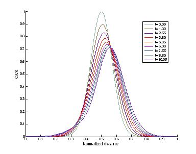 |
Fig. 40.7 Solution of the advection diffusion equation using finite difference |