Now consider the discretized domain as shown in Fig. 40.1. The i is the column number which represents the spatial discritization of the domain. Similarly n is the row number which represents the time discretization. As discussed in Lecture No. 14, we can discretize the diffusion equation as follows.
![]() (40.17)
(40.17)
![]() (40.18)
(40.18)
Putting (40.17) and (40.18) in (40.13), we have
![]() (40.19)
(40.19)
| This is an explicit finite difference form of the equation (40.13). The equation (40.19) can be used to obtain the concentration at different time steps using iterative procedure as shown in Fig. 40.2. The iteration can be performed using any prgramming language. For C0=0, the solution of the one dimensional diffusion equation can be obtained using the following Matlab code. |
|
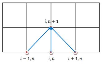 Fig. 40.2 Iterative procedure
 ![Text Box: clear all; % Define the input parameters miu = 0.5; sigma = 0.07; delx = 0.01; delt = 0.00001; %%%%%%%%%%%%%%%%%%%%%%%%%%%%% x = 0:delx:1; % Spatial discretization of the domain t=0:delt:0.03; % Time discretization of the domain [mx nx]=size(x); % Size of x [mt nt]=size(t); % Size of t C = zeros(nx,nt); % Initializing C % Initial condition: Normally distributed concentration for i=2:nx-1 C(i,1) = (1/sqrt(2*pi*sigma^2))*exp(-(x(i)-miu)^2/(2*sigma^2)) ; end C1=max(max(C)); % Main finite difference iteration for n=2:nt for i=2:nx-1 C(i,n) = C(i,n-1)+(delt/delx^2)*(C(i+1,n-1)-2*C(i,n-1)+C(i-1,n-1)); end end C=C/C1; % Generating concentration distribution plot hold on; for t=1:500:nt plot(x,C(:,t), 'color',[rand rand rand]); end axis tight; xlabel('Normalize distance'); ylabel('C/Co'); M=delt*(1:500:nt); M = num2str(M'); legend(M); %%%%%%%%%%%%%%%%%%%%%%%%%%%%%%%%%%%%%%%%%%](images/016.png)
The solutions obtained using the code are shown in Fig. 40.3.
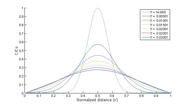 |
Fig. 40.3 Solution of the one dimensional diffusion equation |