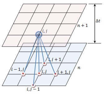
Now consider the discretized domain as shown in Fig. 40.4. The i is the column number which represents the spatial discritization of the domain in x direction. Similarly, j is the row number which represents the spatial discretization in y direction and n is the temporal discretization. Now, we can discretize the diffusion equation as follows.
![]() (40.41)
(40.41)
![]() (40.42)
(40.42)
![]() (40.43)
(40.43)
Putting (40.41), (40.42) and (40.43) in (40.35), we have
![]() (40.44)
(40.44)
| This is the explicit finite difference form of the equation (40.35). The equation (40.44) can be used to obtain the concentration at different time step using iterative procedure as shown in Fig. 40.5. The concentration at (i, j) of time step (n+1)
can be obtained from the known concentration values at
(i−1, j), (i+1, j), (i, j+1), and at (i, j−1) of previous time step (n). The iteration can be performed using any prgramming language. For C0=0, |
|
![Text Box: clear all; % Define the input parameters miux = 0.5; miuy = 0.5; sigmax = 0.07; sigmay = 0.07; delx = 0.01; dely=delx; delt = 0.00001; %%%%%%%%%%%%%%%%%%%%%%%%%%%%% x = 0:delx:1; % Spatial discretization of the domain y = 0:dely:1; % Spatial discretization of the domain t=0:delt:0.01; % Time discretization of the domain [mx nx]=size(x); % Size of x [mx ny]=size(y); % Size of x [mt nt]=size(t); % Size of t C = zeros(nx,ny,nt); % Initializing C % Initial condition: Normally distributed concentration for i=2:nx-1 for j=2:ny-1 C(i,j,1) = (1/sqrt(2*pi*sigmax^2*sigmay^2))*exp(-(x(i)-miux)^2/(2*sigmax^2)-(y(j)-miuy)^2/(2*sigmay^2)) ; end end C1=max(max(max(C))); % Main finite difference iteration for k=2:nt for i=2:nx-1 for j=2:ny-1 C(i,j,k) = C(i,j,k-1)+(delt/delx^2)*(C(i+1,j,k-1)+C(i-1,j,k-1)+C(i,j+1,k-1)+C(i,j-1,k-1)-4*C(i,j,k-1)); end end end C=C/C1; % Generating concentration distribution plot nn=1; for t=1:200:nt figure(nn); surfc(x,y,C(:,:,t)); axis([0 1 0 1 0 1]) xlabel('X'); ylabel('Y'); zlabel('C/Co'); colorbar; shading interp; text(0,1,1.4,num2str(t*delt)); text(-0.1,1,1.44,'t ='); grid on; nn=nn+1; end %%%%%%%%%%%%%%%%%%%%%%%%%%%%%%%%%%%%%%%%%%](images/023.png)
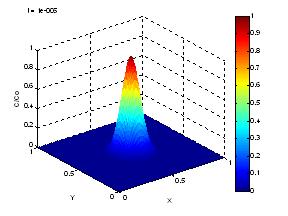
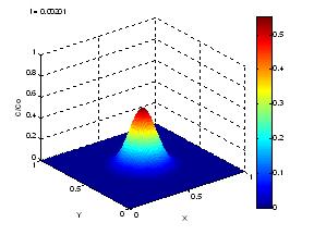
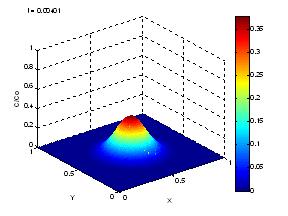
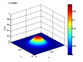
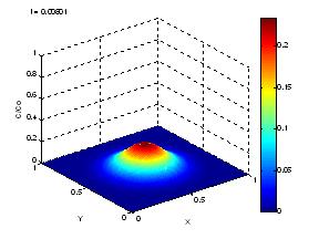
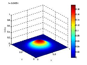
The solutions obtained using the code are shown in Fig. 40.6.
|
Fig. 40.6 Solution of the two dimensional diffusion equation |