Module 8 : Specialized Traffic Studies

Lecture 44 : Congestion Studies

1

2

3

4

5

6

7

8

9

	Congestion pricing Congestion pricing is a method of road user taxation, charging the users of congested roads according to the time spent or distance travelled on those roads. The principle behind congestion pricing is that those who cause congestion or use road in congested period should be charged, thus giving the road user the choice to make a journey or not. Economic principle behind congestion pricing Journey costs include private journey cost, congestion cost, environmental cost, and road maintenance cost. The benefit a road user obtains from the journey is the price he prepared to pay in order to make the journey. As the price gradually increases, a point will be reached when the trip maker considers it not worth performing or it is worth performing by other means. This is known as the critical price. At a cost less than this critical price, he enjoys a net benefit called as consumer surplus(es) and is given by: $$s=x-y$$ (1) where, $x$ is the amount the consumer is prepared to pay, and $y$ is the amount he actually pays. The basics of congestion pricing involves demand function, private cost function as well as marginal cost function. These are explained below. 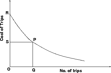Demand Fig. 1 shows the general form of a demand curve. In the figure, area QOSP indicates the absolute utility to trip maker and the area SRP indicates the net benefit. Figure 1: Demand Curve Private cost Total private cost of a trip, is given by: $$c=a+\frac{b}{v}$$ (2) where, $a$ is the component proportional to distance, $b$ is the component proportional to speed, and $v$ is the speed of the vehicle (km/h). In the congested region, the speed of the vehicle can be expressed as, $$v=d-eq$$ (3) where, $q$ is the flow in veh/hour, $d$ and e are constants. Marginal cost Marginal cost is the additional cost of adding one extra vehicle to the traffic stream. It reduces speed and causes congestion and results in increase in cost of overall journey. The total cost incurred by all vehicles in one hour($C_T$) is given by: $$C_T=cq$$ (4) Marginal cost is obtained by differentiating the total cost with respect to the flow($q$) as shown in the following equations. $$M = \frac{d(cq)}{dq} = c+q\frac{dc}{dq}$$ (5) $$\frac{dc}{dq} = \frac{dc}{dv}\times\frac{dv}{dq}$$ (6) $$= (-b)/v^2 \times-e$$ (7) $$= be/v^2$$ (8) $$\frac{d(cq)}{dq} = c+q\frac{dc}{dq}$$ (9) $$= a+\frac{b}{v}+\frac{d-v}{e}\times\frac{be}{v^2}$$ (10) Note that c and q in the above derivation is obtained from Equations 2 and 3 respectively. Therefore the marginal cost is given as: $$M=a+\frac{b}{v}+\frac{(d-v)b}{v^2}$$ (11) Fig. 2 shows the variation of marginal cost per flow as well as private cost per flow. Figure 2: Private cost/flow and cost and marginal curve 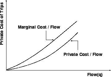It is seen that the marginal cost will always be greater than the private cost, the increase representing the congestion cost. 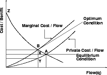Equilibrium condition and Optimum condition Superimposing the demand curve on the private cost/flow and marginal cost/flow curves, the position as shown in Fig. 3 is obtained. The intersection of the demand curve and the private costs curve at point A represents the equilibrium condition, obtained when travel decisions are based on private costs only. The intersection of the demand curve and the marginal costs curve at point B represents the optimum condition. At this point the flow $Q_0$ corresponds to the cost $C_0$ which is the marginal cost as well as the value of the trip to the trip maker. The net benefit under the two positions A and B are shown by the areas ACZ and $BYC_{Y}Z$ respectively. If the conditions are shifted from point A to B, the net benefit due to change will be given by area $CC_{y}YX$ minus AXB. If the area $CC_{y}YX$ is greater than arc AXB, the net benefit will be positive. The shifting of conditions from point A to B can be brought about by imposing a road pricing charge BY. Under this scheme, the private vehicles continuing to use the roads will on an average be worse off in the first place because BY will always exceed the individual increase in benefits XY. Figure 3: Relation between material cost, private cost and demand curves. Numerical example Vehicles are moving on a road at the rate of 500 vehicle/hour, at a velocity of 15 km/hr. Find the equation for marginal cost. Solution: Private cost of the trip is given by, $$c = \frac{a+b}{v}$$ $$= \frac{a+b}{15}$$ It is given that Flow rate, q=500 veh/hr. 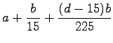Speed of the vehicle is given by, $$v = d-eq$$ $$= d-500e$$ Marginal Cost is given by, $$M = a+\frac{b}{v}+\frac{(d-v)b}{v^2}$$ $$= a+\frac{b}{15}+\frac{(d-15)b}{225}$$ Therefore, the equation of marginal cost for the vehicles moving on the given congested road is given by $M= a+(b/15)+[(d-15)*b/225]$