|
The earliest car-following models considered the difference in speeds between
the leader and the follower as the stimulus.
It was assumed that every driver tends to move with the same speed as that of
the corresponding leading vehicle so that
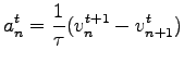 |
(1) |
where  is a parameter that sets the time scale of the model and is a parameter that sets the time scale of the model and
 can be considered as a measure of the sensitivity of the
driver.
According to such models, the driving strategy is to follow the leader and,
therefore, such car-following models are collectively referred to as the follow
the leader model.
Efforts to develop this stimulus function led to five generations of
car-following models, and the most general model is expressed mathematically as
follows. can be considered as a measure of the sensitivity of the
driver.
According to such models, the driving strategy is to follow the leader and,
therefore, such car-following models are collectively referred to as the follow
the leader model.
Efforts to develop this stimulus function led to five generations of
car-following models, and the most general model is expressed mathematically as
follows.
![$\displaystyle a_{n+1}^{t+{\Delta{T}}}={\frac{\alpha_{l,m}~[{v_{n+1}^{t-\Delta{T...
...}-{x_{n+1}^{t-\Delta{T}}}]^l}}{({v_{n}^{t-\Delta{T}}}-{v_{n+1}^{t-\Delta{T}}})}$](img4.png) |
(2) |
where  is a distance headway exponent and can take values from +4 to -1, is a distance headway exponent and can take values from +4 to -1,  is a speed exponent and can take values from -2 to +2, and
  is a
sensitivity coefficient.
These parameters are to be calibrated using field data. is a
sensitivity coefficient.
These parameters are to be calibrated using field data.
|