| |
| | |
|
Let a leader vehicle is moving with zero acceleration for two seconds from time
zero.
Then he accelerates by 1  for 2 seconds, then decelerates by 1for
2 seconds.
The initial speed is 16 m/s and initial location is 28 m from datum.
A vehicle is following this vehicle with initial speed 16 m/s, and position
zero.
Simulate the behavior of the following vehicle using General Motors' Car
following model (acceleration, speed and position) for 7.5 seconds.
Assume the parameters l=1, m=0 , sensitivity coefficient ( for 2 seconds, then decelerates by 1for
2 seconds.
The initial speed is 16 m/s and initial location is 28 m from datum.
A vehicle is following this vehicle with initial speed 16 m/s, and position
zero.
Simulate the behavior of the following vehicle using General Motors' Car
following model (acceleration, speed and position) for 7.5 seconds.
Assume the parameters l=1, m=0 , sensitivity coefficient (
 ) = 13,
reaction time as 1 second and scan interval as 0.5 seconds.
The first column shows the time in seconds.
Column 2, 3, and 4 shows the acceleration, velocity and distance of the leader
vehicle.
Column 5,6, and 7 shows the acceleration, velocity and distance of the follower
vehicle.
Column 8 gives the difference in velocities between the leader and follower
vehicle denoted as ) = 13,
reaction time as 1 second and scan interval as 0.5 seconds.
The first column shows the time in seconds.
Column 2, 3, and 4 shows the acceleration, velocity and distance of the leader
vehicle.
Column 5,6, and 7 shows the acceleration, velocity and distance of the follower
vehicle.
Column 8 gives the difference in velocities between the leader and follower
vehicle denoted as  .
Column 9 gives the difference in displacement between the leader and follower
vehicle denoted as .
Column 9 gives the difference in displacement between the leader and follower
vehicle denoted as  .
Note that the values are assumed to be the state at the beginning of that time
interval.
At time t=0, leader vehicle has a velocity of 16 m/s and located at a distance
of 28 m from a datum.
The follower vehicle is also having the same velocity of 16 m/s and located at
the datum.
Since the velocity is same for both, = 0.
At time t = 0, the leader vehicle is having acceleration zero, and hence has
the same speed.
The location of the leader vehicle can be found out from equation as, x = 28+16 .
Note that the values are assumed to be the state at the beginning of that time
interval.
At time t=0, leader vehicle has a velocity of 16 m/s and located at a distance
of 28 m from a datum.
The follower vehicle is also having the same velocity of 16 m/s and located at
the datum.
Since the velocity is same for both, = 0.
At time t = 0, the leader vehicle is having acceleration zero, and hence has
the same speed.
The location of the leader vehicle can be found out from equation as, x = 28+16 0.5 = 36 m.
Similarly, the follower vehicle is not accelerating and is maintaining the same
speed.
The location of the follower vehicle is, x = 0+160.5 = 8 m.
Therefore, = 36-8 =28m.
These steps are repeated till t = 1.5 seconds.
At time t = 2 seconds, leader vehicle accelerates at the rate of 1 and
continues to accelerate for 2 seconds. After that it decelerates for a period
of two seconds.
At t= 2.5 seconds, velocity of leader vehicle changes to 16.5 m/s.
Thus becomes 0.5 m/s at 2.5 seconds.
also changes since the position of leader changes.
Since the reaction time is 1 second, the follower will react to the leader's
change in acceleration at 2.0 seconds only after 3 seconds.
Therefore, at t=3.5 seconds, the follower responds to the leaders change in
acceleration given by equation i.e., a = 0.5 = 36 m.
Similarly, the follower vehicle is not accelerating and is maintaining the same
speed.
The location of the follower vehicle is, x = 0+160.5 = 8 m.
Therefore, = 36-8 =28m.
These steps are repeated till t = 1.5 seconds.
At time t = 2 seconds, leader vehicle accelerates at the rate of 1 and
continues to accelerate for 2 seconds. After that it decelerates for a period
of two seconds.
At t= 2.5 seconds, velocity of leader vehicle changes to 16.5 m/s.
Thus becomes 0.5 m/s at 2.5 seconds.
also changes since the position of leader changes.
Since the reaction time is 1 second, the follower will react to the leader's
change in acceleration at 2.0 seconds only after 3 seconds.
Therefore, at t=3.5 seconds, the follower responds to the leaders change in
acceleration given by equation i.e., a =
 = 0.23 .
That is the current acceleration of the follower vehicle depends on and
reaction time = 0.23 .
That is the current acceleration of the follower vehicle depends on and
reaction time  of 1 second.
The follower will change the speed at the next time interval. i.e., at time t =
4 seconds.
The speed of the follower vehicle at t = 4 seconds is given by
equation as v= 16+0.2310.5 = 16.12
The location of the follower vehicle at t = 4 seconds is given by
equation as x =
56+160.5+ of 1 second.
The follower will change the speed at the next time interval. i.e., at time t =
4 seconds.
The speed of the follower vehicle at t = 4 seconds is given by
equation as v= 16+0.2310.5 = 16.12
The location of the follower vehicle at t = 4 seconds is given by
equation as x =
56+160.5+
 0.231 0.231
 = 64.03
These steps are followed for all the cells of the table. = 64.03
These steps are followed for all the cells of the table.
Table 1:
Car-following example
 |
 |
 |
 |
|
|
|
|
|
| (1) |
(2) |
(3) |
(4) |
(5) |
(6) |
(7) |
(8) |
(9) |
|
|
|
|
|
|
|
|
|
| 0.00 |
0.00 |
16.00 |
28.00 |
0.00 |
16.00 |
0.00 |
0.00 |
28.00 |
| 0.50 |
0.00 |
16.00 |
36.00 |
0.00 |
16.00 |
8.00 |
0.00 |
28.00 |
| 1.00 |
0.00 |
16.00 |
44.00 |
0.00 |
16.00 |
16.00 |
0.00 |
28.00 |
| 1.50 |
0.00 |
16.00 |
52.00 |
0.00 |
16.00 |
24.00 |
0.00 |
28.00 |
| 2.00 |
1.00 |
16.00 |
60.00 |
0.00 |
16.00 |
32.00 |
0.00 |
28.00 |
| 2.50 |
1.00 |
16.50 |
68.13 |
0.00 |
16.00 |
40.00 |
0.50 |
28.13 |
| 3.00 |
1.00 |
17.00 |
76.50 |
0.00 |
16.00 |
48.00 |
1.00 |
28.50 |
| 3.50 |
1.00 |
17.50 |
85.13 |
0.23 |
16.00 |
56.00 |
1.50 |
29.13 |
| 4.00 |
-1.00 |
18.00 |
94.00 |
0.46 |
16.12 |
64.03 |
1.88 |
29.97 |
| 4.50 |
-1.00 |
17.50 |
102.88 |
0.67 |
16.34 |
72.14 |
1.16 |
30.73 |
| 5.00 |
-1.00 |
17.00 |
111.50 |
0.82 |
16.68 |
80.40 |
0.32 |
31.10 |
| 5.50 |
-1.00 |
16.50 |
119.88 |
0.49 |
17.09 |
88.84 |
-0.59 |
31.03 |
| 6.00 |
0.00 |
16.00 |
128.00 |
0.13 |
17.33 |
97.45 |
-1.33 |
30.55 |
| 6.50 |
0.00 |
16.00 |
136.00 |
-0.25 |
17.40 |
106.13 |
-1.40 |
29.87 |
| 7.00 |
0.00 |
16.00 |
144.00 |
-0.57 |
17.28 |
114.80 |
-1.28 |
29.20 |
| 7.50 |
0.00 |
16.00 |
152.00 |
-0.61 |
16.99 |
123.36 |
-0.99 |
28.64 |
| 8.00 |
0.00 |
16.00 |
160.00 |
-0.57 |
16.69 |
131.78 |
-0.69 |
28.22 |
| 8.50 |
0.00 |
16.00 |
168.00 |
-0.45 |
16.40 |
140.06 |
-0.40 |
27.94 |
| 9.00 |
0.00 |
16.00 |
176.00 |
-0.32 |
16.18 |
148.20 |
-0.18 |
27.80 |
| 9.50 |
0.00 |
16.00 |
184.00 |
-0.19 |
16.02 |
156.25 |
-0.02 |
27.75 |
| 10.00 |
0.00 |
16.00 |
192.00 |
-0.08 |
15.93 |
164.24 |
0.07 |
27.76 |
| 10.50 |
0.00 |
16.00 |
200.00 |
-0.01 |
15.88 |
172.19 |
0.12 |
27.81 |
| 11.00 |
0.00 |
16.00 |
208.00 |
0.03 |
15.88 |
180.13 |
0.12 |
27.87 |
| 11.50 |
0.00 |
16.00 |
216.00 |
0.05 |
15.90 |
188.08 |
0.10 |
27.92 |
| 12.00 |
0.00 |
16.00 |
224.00 |
0.06 |
15.92 |
196.03 |
0.08 |
27.97 |
| 12.50 |
0.00 |
16.00 |
232.00 |
0.05 |
15.95 |
204.00 |
0.05 |
28.00 |
| 13.00 |
0.00 |
16.00 |
240.00 |
0.04 |
15.98 |
211.98 |
0.02 |
28.02 |
| 13.50 |
0.00 |
16.00 |
248.00 |
0.02 |
15.99 |
219.98 |
0.01 |
28.02 |
| 14.00 |
0.00 |
16.00 |
256.00 |
0.01 |
16.00 |
227.98 |
0.00 |
28.02 |
| 14.50 |
0.00 |
16.00 |
264.00 |
0.00 |
16.01 |
235.98 |
-0.01 |
28.02 |
| 15.00 |
0.00 |
16.00 |
272.00 |
0.00 |
16.01 |
243.98 |
-0.01 |
28.02 |
| 15.50 |
0.00 |
16.00 |
280.00 |
0.00 |
16.01 |
251.99 |
-0.01 |
28.01 |
| 16.00 |
0.00 |
16.00 |
288.00 |
-0.01 |
16.01 |
260.00 |
-0.01 |
28.00 |
| 16.50 |
0.00 |
16.00 |
296.00 |
0.00 |
16.01 |
268.00 |
-0.01 |
28.00 |
| 17.00 |
0.00 |
16.00 |
304.00 |
0.00 |
16.00 |
276.00 |
0.00 |
28.00 |
| 17.50 |
0.00 |
16.00 |
312.00 |
0.00 |
16.00 |
284.00 |
0.00 |
28.00 |
| 18.00 |
0.00 |
16.00 |
320.00 |
0.00 |
16.00 |
292.00 |
0.00 |
28.00 |
| 18.50 |
0.00 |
16.00 |
328.00 |
0.00 |
16.00 |
300.00 |
0.00 |
28.00 |
| 19.00 |
0.00 |
16.00 |
336.00 |
0.00 |
16.00 |
308.00 |
0.00 |
28.00 |
| 19.50 |
0.00 |
16.00 |
344.00 |
0.00 |
16.00 |
316.00 |
0.00 |
28.00 |
| 20.00 |
0.00 |
16.00 |
352.00 |
0.00 |
16.00 |
324.00 |
0.00 |
28.00 |
| 20.50 |
0.00 |
16.00 |
360.00 |
0.00 |
16.00 |
332.00 |
0.00 |
28.00 |
Figure 1:
Velocity vz Time
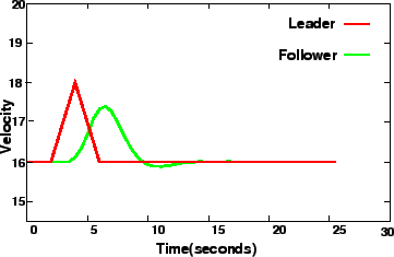 |
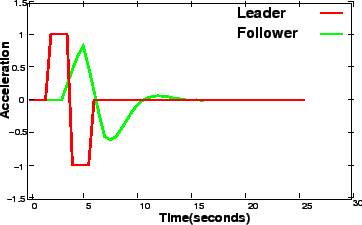
Figure 2:
Acceleration vz Time
 |
|
|
| | |
|
|
|