Here, is called as velocity potential function and its gradient gives rise to velocity vector. The knowledge immediately gives the velocity components. In cartesian coordinates, the velocity potential function can be defined as, so that Eq. (3.3.16) can be written as,

(3.3.17)

So, the velocity components can be written as,

(3.3.18)

In cylindrical coordinates, if , then

(3.3.19)

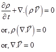
Further, if the flow is incompressible i.e. , then continuity equation can be written as,

(3.3.20)

Therefore, for a flow which is incompressible and irrotational, Eqs. (3.3.16) and (3.3.20) can be combined to yield a second order Laplace equation in a three-dimensional plane.

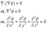(3.3.21)

Thus, any irrotational, incompressible flow has a velocity potential and stream function (for two-dimensional flow) that both satisfy Laplace equation . Conversely, any solution of Laplace equation represents both velocity potential and stream function (two-dimensional) for an irrotational, incompressible flow.

An irrotational flow allows a velocity potential to be defined and leads to simplification of fundamental equations. Instead of dealing with the velocity components u, v and w as unknowns, one can deal with only one parameter , for a given problem. Since, the irrotational flows are best described by velocity potential, such flows are called as potential flows . In these flows, the lines with constant , is known as equipotential lines . In addition, a line drawn in space such that is the tangent at every point is defined as a gradient line and thus can be called as streamline .