Next: Existence of Solution of Up: Linear System of Equations Previous: Elementary Matrices Contents
In previous sections, we solved linear systems using Gauss elimination method or the Gauss-Jordan method. In the examples considered, we have encountered three possibilities, namely
Based on the above possibilities, we have the following definition.
The question arises, as to whether there are conditions under which the linear system
![]() is consistent.
The answer to this question is in the affirmative. To proceed further, we need
a few definitions and remarks.
is consistent.
The answer to this question is in the affirmative. To proceed further, we need
a few definitions and remarks.
Recall that the row reduced echelon form of a matrix is unique and therefore, the number of non-zero rows is a unique number. Also, note that the number of non-zero rows in either the row reduced form or the row reduced echelon form of a matrix are same.
The reader is advised to supply a proof.
Therefore, we can define column-rank of ![]() as the number
of non-zero columns in
as the number
of non-zero columns in ![]() It will be proved later that
It will be proved later that
Thus we are led to the following definition.
 the
the
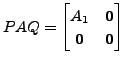
We now apply column operations to the matrix ![]() Let
Let ![]() be the
matrix obtained from
be the
matrix obtained from ![]() by successively interchanging the
by successively interchanging the
![]() and
and
![]() column of
column of ![]() for
for
 Then
the matrix
Then
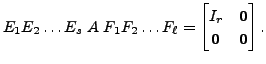
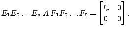
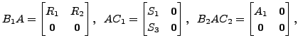
the matrix ![]() can be written in the form
can be written in the form
 where
where ![]() is a matrix of appropriate size. As the
is a matrix of appropriate size. As the
![]() block of
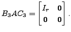
block of ![]() is an identity matrix, the block
is an identity matrix, the block ![]() can
be made the zero matrix by application of column operations to
can
be made the zero matrix by application of column operations to
![]() This gives the required result.
height6pt width 6pt depth 0pt
This gives the required result.
height6pt width 6pt depth 0pt
 Then the system of equations
 Define
![$\displaystyle A Q = \left[\begin{array}{c\vert c} & \\ \star & {\mathbf 0}\\ & \end{array}\right]$](img585.png)
as the elementary martices
 Let
Let
 and
and
 and
and
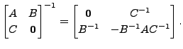
 Also, prove that
the matrix
Also, prove that
the matrix  and
and 
 and
and
 Define
 ]
]
If
and