Next: Determinant Up: Appendix Previous: Appendix Contents
 and
and
 respectively. Suppose
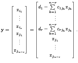
 the set of solutions of the
linear system is an infinite set and has the form
the set of solutions of the
linear system is an infinite set and has the form
where
 the solution set of the linear
system has a unique
the solution set of the linear
system has a unique
 vector
 the linear system has no solution.

Then
![$ [C \; \; {\mathbf d}]$](img479.png) has its first
has its first
![]() rows as the non-zero rows. So, by Remark 2.3.5,
the matrix
rows as the non-zero rows. So, by Remark 2.3.5,
the matrix
![]() has
has ![]() leading columns. Let the leading
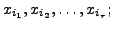
columns be
leading columns. Let the leading
columns be
![]() Then we
observe the following:
Then we
observe the following:
 The entry

 columns correspond to the
 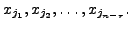 So, the free variables correspond to the columns
 and is the leading term. Also, the first
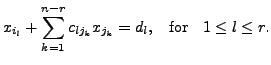
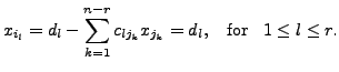
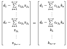
These equations can be rewritten as
Let
 |
(15.1.1) |
 for
for
 are free variables,
let us assign arbitrary constants
are free variables,
let us assign arbitrary constants
 That is, for
 |
|||
 |
 Also, for
 Observe the following:
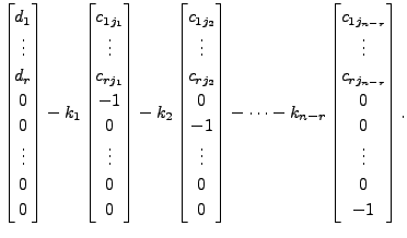
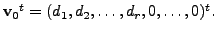
 will
give us the solution vector
will
give us the solution vector
 Suppose that for
 's are
obtained by applying the same
rearrangement to the entries of
's are
obtained by applying the same
rearrangement to the entries of
Thus, we have obtained the desired result for the case

Here the first ![]() rows of the row reduced echelon matrix
rows of the row reduced echelon matrix
![]() are the non-zero rows. Also, the number of columns in
are the non-zero rows. Also, the number of columns in
![]() equals
equals
![]() So, by Remark 2.3.5,
all the columns of
So, by Remark 2.3.5,
all the columns of ![]() are leading columns and all the
variables
are leading columns and all the
variables
![]() are basic variables.
Thus, the row reduced echelon form
are basic variables.
Thus, the row reduced echelon form
![]() of
of
![]() is given by
is given by
![$\displaystyle [C \;\; {\mathbf d}] = \begin{bmatrix}I_n &
\tilde{{\mathbf d}}\\ {\mathbf 0}& {\mathbf 0}\end{bmatrix}.$](img5719.png)
Therefore, the solution set of the linear system

As ![]() has
has ![]() columns, the row reduced echelon matrix
columns, the row reduced echelon matrix
![]() has
has ![]() columns. The condition,
columns. The condition, ![]() implies that
implies that
 We now observe the following:
 implies that the
Thus, for the equivalent linear system
![]() the
the
![]() equation is
equation is
This linear equation has no solution. Hence, in this case, the linear system
We now state a corollary whose proof is immediate from previous results.
A K Lal 2007-09-12