Lecture 4: More on Dependent Sources

Figure 5.1: A dependent Source

All dependent sources are linear elements if (see figure 5.1) K=constant and the output is proportional to controlling variable. Here, in figure 5.1, $V_0=$ effect, and V= cause. If K is constant, $\Delta V$ always gives same $\Delta V_0$ for all values of $V$. $V_0 \propto V_R$. In general all the measured variables can be written as linear combination of all the causes, since nodal voltage or loop current method leads to linear equations. This is true for network with linear elements, and linear dependent sources.

For measuring effect of many sources (also called forcing functions), the effect due to one source at a time is computed (assuming all others to be null). For the sources to be nullified means that if they are voltages sources, they are short circuited (making the voltage of source zero), and if they are current sources, they are open circuited (making the current from the source zero). Effects of all individual independent sources are added to get effect due to presence of all the independent sources. This is known as Superposition Theorem and is valid because of linearity in the circuit (as explained above).

While applying superposition theorm, depenendent sources are retained as any other circuit element. They should not be nullified to get their effect separately on the quantity of interest.

Example: Consider the circuit shown in figure 5.2

Figure 5.2: Example Circuit

Using loop analyis, as shown in fig5.3, we apply KVL. For $i_1=2 \; A$.

Figure 5.3: Tree for the example circuit

$$2-(i_1+i_2)\times 1 -i_2 \times 2 -3(i_1+i_2)=0$$

$$-i_2-2i_2 -6-3i_2=0$$

$$i_2=-1\;A$$

Solving the same circuit using superposition theorem

There are two sources. We will take one at a time and find the contribution in $i$ shown in figure which is quantity of interest for us. Taking Voltage source first (as in figure 5.4)

Figure 5.4: Taking Voltage source

$$i_a=\frac{1}{3}\;Amp$$ (5.1)

Taking current source only, (as in figure 5.5), making tree (as in figure 5.6)

Figure 5.5: Taking Current Source only

Figure 5.6: Making Tree for the circuit considering current source only

$$i_2=2\;A$$

$$i_1(1+3)+(i_1-i_2)2=0$$

$$4i_1+2i_1-4=0$$

$$i_1=\frac{2}{3}$$

$$i_b=\frac{-4}{3}\; A$$

$$i_a + i_b = -1 \; A$$

When one is finding effect of an independent source, other independent sources are nullified. Let's take an example having dependent source (Fig.7.5).

Figure 5.7: Circuit for analysis with dependent source

Taking voltage source first (Fig.7.6)

Figure 5.8: Taking only voltage source

Using KVL:$i_a=i$

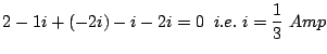$$2-1i+(-2i)-i -2i=0\;\;i.e.\;i=\frac{1}{3}\;Amp$$ (5.2)

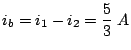
Taking Current source (Fig.7.7), and making a tree (Fig.7.8), we write KVL and solve

Figure 5.9: Taking Current Source

Figure 5.10: Making a tree

$$-i_13+(-2i_1)-(i_1-i_2)1=0$$

$$-6i_1+i_2=0$$

$$i_2=-2 \; A$$

$$i_1=\frac{-1}{3}\;A$$

$$i_b=i_1-i_2=\frac{5}{3}\;A$$

$$i_a+i_b=\frac{6}{3}=2\;A$$

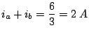Now we verify the solution from loop current method directly (Fig.7.9). Making tree (Fig.7.10).

Figure 5.11: Direct Verification

Figure 5.12: Making Tree

$$i_2=-2\;Amp$$

$$KVL\;for\;loop\;1: 2-i_1-2i_1-(i_1-i_2)-2i_1=0$$

$$-6i_1+i_2 +2=0$$

$$Hence \; i_1=0$$

$$i_1-i_2=?$$

$$0-(-2)=2\;Amp$$

which is correct answer.