For the forward whirl we have , hence equation (b) reduces to

(c)

which can be solved as

(d)

Negative value is not a feasible solution, taking positive value only, we get

Hence only single forward critical speed is possible. For the backward whirl, we have , hence from equation (b), we get

(e)

which can be solved to give two positive roots, as

(f)

Hence two possible backward critical speeds are possible

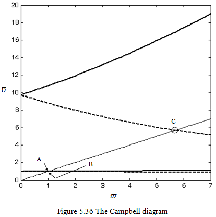
Figure 5.36 shows the corresponding Campbell diagram, which can be drawn with the equation (b) of the following form

(g)

In Figure 5.36, forward whirl natural frequencies are drawn with solid lines and backward whirl by dashed lines. Locations of critical speeds are: A(1.007, 1.007), B(0.9787, -0.9787), C(5.7091, -5.7091). It can be seen that coordinates of three intersection points, between natural whirl frequency curves and a line  matches with critical speed ratios obtained in equations (d) and (f) and there is no intersection corresponding to the negative root in equation (d).

Example 5.5 Obtain the forward and backward synchronous transverse critical speeds for a general motion of a rotor as shown in Figure 5.37. The rotor is assumed to be fixed supported at one end. Take the mass of the disc m = 2 kg, the polar mass moment of inertia I_p = 0.01 kg-m² and the diametral moment of inertia I_d = 0.005 kg-m². The shaft is assumed to be massless, and its length and diameter are 0.2 m and 0.1 m, respectively. Take the shaft Young’s modulus E = 2.1 X 10¹¹ N/m². Draw the Campbell diagram and show. the forward and backward synchronous transverse critical speeds 

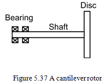
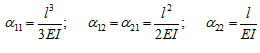
Solution: For the cantilever beam, influence coefficients are related as

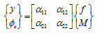
With

Solution: The frequency equation is

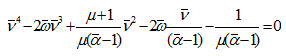(a)

From the given parameters, we have

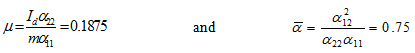(b)

On  substituting equations (b) into equation (a), we  get

(c)

For the forward whirl we have = +, hence equation (c) becomes

(d)

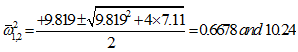
On solving equation (d), we will get the roots as

(e)

Negative value is not a feasible solution, taking positive value only, then we get

(f)

Hence, only single forward critical speed is possible.

For the backward whirl, we have = -,  on substituting in equation (c), we get

(g)

which gives

(h)

or

(i)

Hence, the possible backward critical speeds are

(j)

To summarise the forward and backward critical speeds are given as

(k)

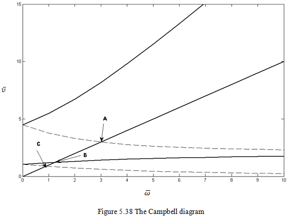
Campbell diagram: We can draw the Campbell diagram from the below equation (c), as

(l)

In Figure 5.38, on x-axis we have taken  and on y-axis we have taken . Forward whirl natural frequencies are drawn with solid lines and backward whirl frequencies are drawn with dotted lines. From the diagram it can be seen that coordinates of intersection points (A(2.97, 2.97), B(1.21, 1.21), C(0.84, 0.84) ), between natural whirl curves and a line =  matches with critical speed ratio obtained in equations (e) and (i) and there is no intersection corresponding to the negative root in equation in (e).