2.3 Controller with Observer
The observer dynamics:
![]()
Combining with the system dynamics
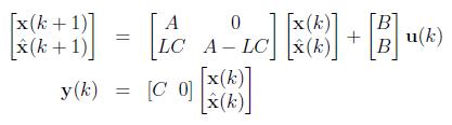
Since the states are unavailable for measurements, the control input is
![]()
Putting the control law in the augmented equation
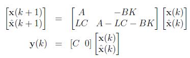
The error dynamics is
![]()
If we augment the above with the system dynamics, we get
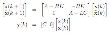
where the dimension of the augmented system matrix is R2nx2n . Looking at the matrix one can easily understand that 2n eigenvalues of the augmented matrix are equal to the individual eigenvalues of ![]() and
and ![]() .
.
Conclusion: We can reach to a conclusion from the above fact is the design of control law, i.e., ![]() is separated from the design of the observer, i.e.,
is separated from the design of the observer, i.e., ![]() .
.
The above conclusion is commonly referred to as separation principle .
The block diagram of controller with observer is shown in Figure 3.
![\begin{figure}\centering
\begin{pspicture}(-2,-2)(12,8)
%\pnode(-1,6){u}\rput(...
...B=180]{-}{u1}{a2}
\rput(4,-0.7){$\mathbf{u}(k)$}
\end{pspicture}
\end{figure}](images/img72.png)