Computation of observer gain matrix L
The task is to place the poles of ![]() . Necessary and sufficient condition for arbitrary pole placement is that the pair should be controllable.
. Necessary and sufficient condition for arbitrary pole placement is that the pair should be controllable.
Assumption: The pair ![]() is observable. Thus, from the theorem of duality, the pair
is observable. Thus, from the theorem of duality, the pair ![]() is controllable.
is controllable.
You should note that the eigenvalues of ![]() are same as that of
are same as that of ![]() . It is same as a hypothetical pole placement problem for the system
. It is same as a hypothetical pole placement problem for the system ![]() , using a control law
, using a control law ![]() .
.
Example:
The observability matrix
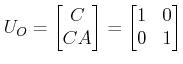
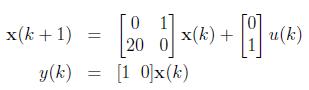
is non singular. Thus the pair![]() is observable. The observer dynamics are
is observable. The observer dynamics are
![]()
L should be designed such that the observer poles are at 0.2 and 0.3.
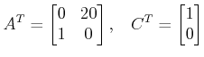
We design LT such that ![]() has eigenvalues at 0.2 and 0.3.
has eigenvalues at 0.2 and 0.3.
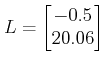
Using Ackermann's formula, ![]() . Thus
. Thus