Let ![]() be the estimation error. Then the error dynamics are defined by
be the estimation error. Then the error dynamics are defined by
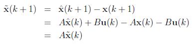
with the initial estimation error as ![]() If the eigenvalues of A are inside the unit circle then
If the eigenvalues of A are inside the unit circle then ![]() will converge to 0 . But we have no control over the convergence rate.
will converge to 0 . But we have no control over the convergence rate.
Moreover, A may have eigenvalues outside the unit circle. In that case ![]() will diverge from 0 . Thus the open loop estimator is impractical.
will diverge from 0 . Thus the open loop estimator is impractical.
2.2 Luenberger State Observer
Consider the system ![]() . Luenberger observer is shown in Figure 2. The observer dynamics can be expressed as:
. Luenberger observer is shown in Figure 2. The observer dynamics can be expressed as:
| (1) |
![\begin{figure}\centering \begin{pspicture}(-2,0)(12,8) \pnode(-1,6){u}\rput(-1... ...eA=180,angleB=-90]{->}{G7}{S2}\ncline{->}{G5}{yh} \end{pspicture} \end{figure}](images/img32.png) |
Figure 2: Luenberger observer
The closed loop error dynamics can be derived as:
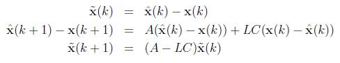
It can be seen that ![]() , if L can be designed such that
, if L can be designed such that ![]() has eigenvalues inside the unit circle of z -plane.
has eigenvalues inside the unit circle of z -plane.
The convergence rate can also be controlled by properly choosing the closed loop eigenvalues.