The controllability matrix

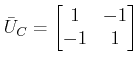
$\displaystyle \bar U_C= \begin{bmatrix}1 & -1 \\ -1 & 1 \end{bmatrix}$

implies that the state model is uncontrollable. The observability matrix

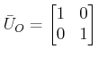
$\displaystyle \bar U_O= \begin{bmatrix}1 & 0 \\ 0 & 1 \end{bmatrix}$

implies that the state model is observable. The system difference equation will result in a tranfer function which would involve pole-zero cancellation. Whenever there is a pole zero cancellation, the state space model will be either uncontrollable or unobservable or both.

4 Controllability/Observability after sampling

Question: If a continuous time system is undergone a sampling process will its controllability or observability property be maintained?

The answer to the question depends on the sampling period T and the location of the eigenvalues of A.

. Loss of controllability and/or observability occurs only in presence of oscillatory modes of the system.

. A sufficient condition for the discrete model with sampling period T to be controllable is that whenever $Re[\lambda_i - \lambda_j]=0$ , $\vert Im[\lambda_i-\lambda_j]\vert \ne 2\pi m/T$ for

. The above is also a necessary condition for a single input case.

Note: If a continuous time system is not controllable or observable, then its discrete time version, with any sampling period, is not controllable or observable.