This implies that the output response is deadbeat only at sampling instants. However, the true output c(t) has inter sampling ripples which makes the system response as shown in Figure 2.

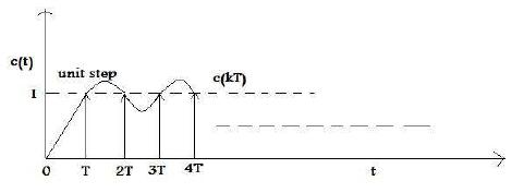
Figure 2: Rippled output response for Example 1

Thus the system takes forever to reach its steady state. The necessary and sufficient condition for c(t) to track a unit step input in finite time is

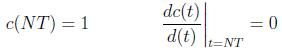
$\displaystyle c(NT) = 1\,\,\,\,\,\,\,\,\,\,\,\,\,\,\,\,\,\,\,\,\,\,\left. {\frac{{dc(t)}}{{d(t)}}} \right\vert _{t = NT} = 0$

for finite N and all the higher derivatives should equal to zero. Let

$\displaystyle w(t) = \frac{{dc(t)}}{{d(t)}}$

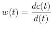
Taking z -transform,

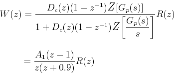
$\begin{displaymath} \begin{array}{l} W(z) = \dfrac{{D_c(z)(1 - z^{ - 1} )\tex... ...\, = \dfrac{{A_1(z - 1)}}{{z(z + 0.9)}}R(z) \\ \end{array} \end{displaymath}$

where A₁ is a constant. Unit step response of W(z) will not go to zero in finite time since poles of $\dfrac{{W(z)}}{{R(z)}}$ are not all at z = 0.

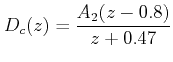
If we now apply the condition that zero of $G_{h0} G_p (z)$ at z = - 0.9 should not be canceled by D_c(z) , then

$\displaystyle M(z) = (1 + 0.9z^{ - 1} )m_1 z^{ - 1}$

$\displaystyle 1 - M(z) = (1 - z^{ - 1} )(1 + a_1 z^{ - 1} )$

Solving

$\displaystyle \Rightarrow m_1 = 0.5,\,\,\,\,\,\,\,\,\,\,\,\,\,\,\,\,a_1 = 0.5$

Thus

$\displaystyle M(z) = \frac{{0.5(z + 0.9)}}{{z^2 }}$

$\displaystyle D_c (z) = \frac{{a_2(z - 0.8)}}{{z + 0.5}}$

$\displaystyle C(z) = a_3z^{ - 1} + z^{ - 2} + z^{ - 3} + .......$

where A₂ and A₃ are constants. This implies that the dead beat response reaches the steady state after two sampling periods.