Nyquist plot of GH(z), as shown in Figure 3, intersects the negative real axis at -0.025K when 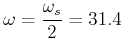 rad/sec.
![]() can be computed as
can be computed as
![]()
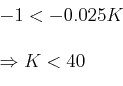
It can be seen from Figure 3 that for ![]() to be -90°, (-1, j 0) point should be located at the left of -0.025K point. Thus for stability
to be -90°, (-1, j 0) point should be located at the left of -0.025K point. Thus for stability
If K > 40, (-1, j 0) will be at the right of ![]() point, hence making
point, hence making ![]() .
.
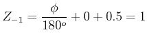
If ![]() , we get from (1)
, we get from (1)
Thus for K > 40, one of the closed loop poles will be outside the unit circle.
If K is negative we can still use the same Nyquist plot but refer (+1, j0 ) point as the critical point. ![]() in this case still equals +90° and the system is unstable. Hence the stable range of K is 0 ≤ K < 40
in this case still equals +90° and the system is unstable. Hence the stable range of K is 0 ≤ K < 40
More details can be found in Digital Control Systems by B. C. Kuo.