Now let us denote the angle traversed by the phasor drawn from (-1, j0) point to the Nyquist plot of GH(z) as ω varies from $\dfrac{\omega_s}{2}$ to 0 , on the unit circle of z1 excluding the small indentations, by $\phi$ .

It can be shown that

$\displaystyle \phi = (Z_{ - 1} - P_{ - 1} - 0.5P_0 )180^0$

(1)

For the closed loop digital control system to be stable, Z_-1 should be equal to zero. Thus the Nyquist criterion for stability of the closed loop digital control systems is

$\displaystyle \phi = - (P_{ - 1} + 0.5P_0 )180^0$

(2)

Hence, we can conclude that for the closed loop digital control system to be stable, the angle, traversed by the phasor drawn to the GH(z) plot from (-1, j0) point as ω varies from $\dfrac{\omega_s}{2}$ to 0 , must satisfy equation (2).

Example 1: Consider a digital control system for which the loop transfer function is given as

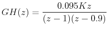
$\displaystyle GH(z) = \frac{{0.095Kz}}{{(z - 1)(z - 0.9)}}$

where K is a gain parameter. The sampling time T = 0.1 sec.

Since GH(z) has one pole on the unit circle and does not have any pole outside the unit circle, P_-1 = 0 and P₀ = 1
Nyquist path has a small indentation at z =1 on the unit circle. The Nyquist plot is shown in Figure 3.

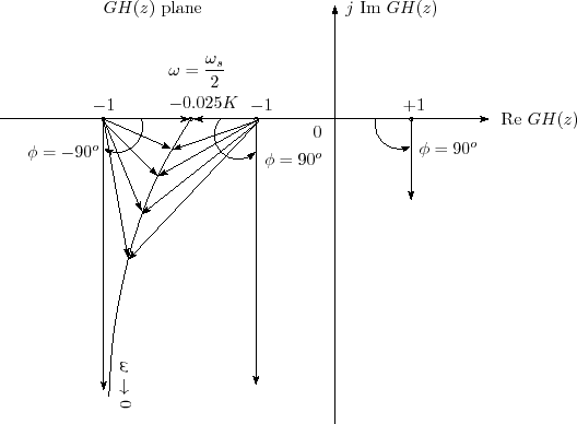$\begin{figure} \centering \input{m5l4fig1.pstex_t} \end{figure}$

Figure 3: Nyquist plot for Example 1