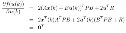
Taking derivative of the above function with respect to u(k),

The matrix ${B^T}PB + R$ is positive definite since R is positive definite, thus it is invertible. Hence,

$\displaystyle \boldsymbol{u}^*(k)= -({B^T}PB + R)^{-1}B^TPA \boldsymbol{x}(k) = -K \boldsymbol{x}(k)$

where $K=({B^T}PB + R)^{-1}B^TPA$ . Let us denote ${B^T}PB + R$ by S. Thus

$\displaystyle \boldsymbol{u}^*(k)=-S^{-1} B^TPA \boldsymbol{x}(k)$

We will now check whether or not u* satisfies the second order sufficient condition for minimization. Since

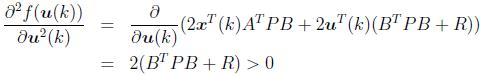
u* satisfies the second order sufficient condition to minimize f.

The optimal controller can thus be constructed if an appropriate Lyapunov matrix P is found. For that let us first find the closed loop system after introduction of the optimal controller.

$\displaystyle \boldsymbol{x}(k + 1) = (A-BS^{-1}B^TPA)\boldsymbol{x}(k)$

Since the controller satisfies the hypothesis of the theorem, discussed in the previous lecture,

$\displaystyle \boldsymbol{x}^T(k + 1)P \boldsymbol{x}(k + 1)-\boldsymbol{x}^T(k... ...mbol{x}^T}(k)Q\boldsymbol{x}(k) + {\boldsymbol{u}^*}^T(k)R\boldsymbol{u}^*(k)=0$

Putting the expression of u* in the above equation,

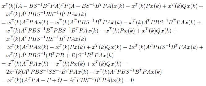
The above equation should hold for any value of x(k). Thus

$\displaystyle A^TPA - P + Q - A^TPBS^{-1}B^TPA=0$

which is the well known discrete Algebraic Riccati Equation (ARE). By solving this equation we can get P to form the optimal regulator to minimize a given quadratic performance index.