1 Linear Quadratic Regulator
Consider a linear system modeled by
![]()
where ![]() and
and ![]() . The pair
. The pair ![]() is controllable.
is controllable.
The objective is to design a stabilizing linear state feedback controller ![]() which will minimize the quadratic performance index, given by,
which will minimize the quadratic performance index, given by,
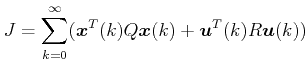
where, ![]() and
and ![]() . Such a controller is denoted by u*.
. Such a controller is denoted by u*.
We first assume that a linear state feedback optimal controller exists such that the closed loop system
![]()
is asymptotically stable.
This assumption implies that there exists a Lyapunov function ![]() for the closed loop system, for which the forward difference
for the closed loop system, for which the forward difference
![]()
is negative definite.
We will now use the theorem as discussed in the previous lecture which says if the controller u* is optimal, then
![]()
Now, finding an optimal controller implies that we have to find an appropriate Lyapunov function which is then used to construct the optimal controller.
Let us first find the u* that minimizes the function
![]()
If we substitute ![]() in the above expression, we get
in the above expression, we get
