Equation (5) is known as the discrete Euler-Lagrange equation and equation (6) is called the transversality condition which is nothing but the boundary condition needed to solve equation (5).

Discrete Euler-Lagrange equation is the necessary condition that must be satisfied for J_a to be an extremal.

With reference to the additional conditions (2) and (3), for arbitrary $\boldsymbol{\mu}(k)$ and $\boldsymbol{\nu}(k+1)$ ,

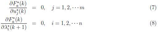
Equation (8) leads to

$\displaystyle \boldsymbol{x}^*(k + 1) = f(k, \boldsymbol{x}^*(k), \boldsymbol{u}^*(k))$

which means that the state equation should satisfy the optimal trajectory. Equation (7) gives the optimal control $\boldsymbol{u}^*(k)$ in terms of $\boldsymbol{\lambda}^*(k+1)$

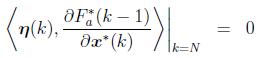
In a variety of the design problems, the initial state x(0) is given. Thus η (0) = 0 since x(0) is fixed. Hence the tranversality condition reduces to

Again, a number of optimal control problems are classified according to the final conditions.

If x(N) is given and fixed, the problem is known as fixed-endpoint design. On the other hand, if x(N) is free, the problem is called a free endpoint design.

For fixed endpoint (x(N) = fixed, η (N) = 0 ) problems, no transversality condition is required to solve.

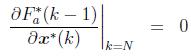
For free endpoint the transversality condition is given as follows.

For more details, one can consult Digital Control Systems by B. C. Kuo.